Price Swaptions with Interest-Rate Models Using Simulation
Introduction
This example shows how to price European swaptions using interest-rate models in Financial Instruments Toolbox™. Specifically, a Hull-White one factor model, a Linear Gaussian two-factor model, and a LIBOR Market Model are calibrated to market data and then used to generate interest-rate paths using Monte Carlo simulation.
The following sections set up the data that is then used with examples for Simulate Interest-Rate Paths Using the Hull-White One-Factor Model, Simulate Interest-Rate Paths Using the Linear Gaussian Two-Factor Model, and Simulate Interest-Rate Paths Using the LIBOR Market Model:
Construct a Zero Curve
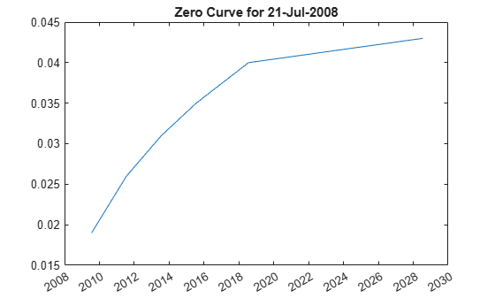
This example shows how to use ZeroRates for a zero curve that is hard-coded. You can also create a zero curve by bootstrapping the zero curve from market data (for example, deposits, futures/forwards, and swaps)
The hard-coded data for the zero curve is defined as:
Settle = datetime(2008,7,21);

% Zero Curve
CurveDates = daysadd(Settle,360*([1 3 5 7 10 20]),1);
ZeroRates = [1.9 2.6 3.1 3.5 4 4.3]'/100;

plot(CurveDates,ZeroRates)
datetick
title(['Zero Curve for ' datestr(Settle)]);
Construct an IRDataCurve object.
irdc = IRDataCurve('Zero',Settle,CurveDates,ZeroRates);Create the RateSpec using intenvset.
RateSpec = intenvset('Rates',ZeroRates,'EndDates',CurveDates,'StartDate',Settle)
RateSpec = struct with fields:
           FinObj: 'RateSpec'
      Compounding: 2
             Disc: [6×1 double]
            Rates: [6×1 double]
         EndTimes: [6×1 double]
       StartTimes: [6×1 double]
         EndDates: [6×1 double]
       StartDates: 733610
    ValuationDate: 733610
            Basis: 0
     EndMonthRule: 1
Define Swaption Parameters
While Monte Carlo simulation is typically used to value more sophisticated derivatives (for example, Bermudan swaptions), in this example, the price of a European swaption is computed with an exercise date of five years and an underlying swap of five years.
InstrumentExerciseDate = datenum('21-Jul-2013');
InstrumentMaturity = datenum('21-Jul-2018');
InstrumentStrike = .045;
Compute the Black Model and the Swaption Volatility Matrix
Black's model is often used to price and quote European exercise interest-rate options, that is, caps, floors and swaptions. In the case of swaptions, Black's model is used to imply a volatility given the current observed market price. The following matrix shows the Black implied volatility for a range of swaption exercise dates (columns) and underlying swap maturities (rows).
SwaptionBlackVol = [22 21 19 17 15 13 12
    21 19 17 16 15 13 11
    20 18 16 15 14 12 11
    19 17 15 14 13 12 10
    18 16 14 13 12 11 10
    15 14 13 12 12 11 10
    13 13 12 11 11 10 9]/100;
ExerciseDates = [1:5 7 10];
Tenors = [1:5 7 10];

EurExDatesFull = repmat(daysadd(Settle,ExerciseDates*360,1)',...
    length(Tenors),1);
EurMatFull = reshape(daysadd(EurExDatesFull,...
    repmat(360*Tenors,1,length(ExerciseDates)),1),size(EurExDatesFull));
Select Calibration Instruments
Selecting the instruments to calibrate the model to is one of the tasks in calibration. For Bermudan swaptions, it is typical to calibrate to European swaptions that are co-terminal with the Bermudan swaption to be priced. In this case, all swaptions having an underlying tenor that matures before the maturity of the swaption to be priced (21-Jul-2018) are used in the calibration.
% Find the swaptions that expire on or before the maturity date of the
% sample swaption
relidx = find(EurMatFull <= InstrumentMaturity);
Compute Swaption Prices Using Black's Model
This example shows how to compute swaption prices using Black's Model. The swaption prices are then used to compare the model’s predicted values that are obtained from the calibration process.
To compute the swaption prices using Black's model:
SwaptionBlackPrices = zeros(size(SwaptionBlackVol));
SwaptionStrike = zeros(size(SwaptionBlackVol));

for iSwaption=1:length(ExerciseDates)
    for iTenor=1:length(Tenors)
        [~,SwaptionStrike(iTenor,iSwaption)] = swapbyzero(RateSpec,[NaN 0], Settle, EurMatFull(iTenor,iSwaption),...
            'StartDate',EurExDatesFull(iTenor,iSwaption),'LegReset',[1 1]);
        SwaptionBlackPrices(iTenor,iSwaption) = swaptionbyblk(RateSpec, 'call', SwaptionStrike(iTenor,iSwaption),Settle, ...
            EurExDatesFull(iTenor,iSwaption), EurMatFull(iTenor,iSwaption), SwaptionBlackVol(iTenor,iSwaption));
    end
end
Define Simulation Parameters
This example shows how to use the
simTermStructs method with
HullWhite1F, LinearGaussian2F, and
LiborMarketModel objects.
To demonstrate using the simTermStructs method with
HullWhite1F, LinearGaussian2F, and
LiborMarketModel objects, use the following
simulation
parameters:
nPeriods = 5;
DeltaTime = 1;
nTrials = 1000;

Tenor = (1:10)';

SimDates = daysadd(Settle,360*DeltaTime*(0:nPeriods),1)
SimTimes = diff(yearfrac(SimDates(1),SimDates))

% For 1 year periods and an evenly spaced tenor, the exercise row will be
% the 5th row and the swaption maturity will be the 5th column
exRow = 5;
endCol = 5;
SimDates =

      733610
      733975
      734340
      734705
      735071
      735436


SimTimes =

    1.0000
    1.0000
    1.0000
    1.0027
    1.0000
Simulate Interest-Rate Paths Using the Hull-White One-Factor Model
This example shows how to simulate interest-rate paths using
the Hull-White one-factor model. Before beginning this example that uses a
HullWhite1F model, make sure that you have set up the
data as described in:
The Hull-White one-factor model describes the evolution of the short rate and is specified using the zero curve, alpha, and sigma parameters for the equation
where:
dr is the change in the short-term interest rate over a small interval, dt.
r is the short-term interest rate.
Θ(t) is a function of time determining the average direction in which r moves, chosen such that movements in r are consistent with today's zero coupon yield curve.
α is the mean reversion rate.
dt is a small change in time.
σ is the annual standard deviation of the short rate.
W is the Brownian motion.
The Hull-White model is calibrated using the function
swaptionbyhw, which constructs a trinomial tree to price
the swaptions. Calibration consists of minimizing the difference between the
observed market prices (computed above using the Black's implied swaption
volatility matrix, see Compute the Black Model and the Swaption Volatility Matrix) and the model’s
predicted prices.
In this example, the Optimization Toolbox™ function lsqnonlin is used to find the
parameter set that minimizes the difference between the observed and predicted
values. However, other approaches (for example, simulated annealing) may be
appropriate. Starting parameters and constraints for α and
σ are set in the variables x0,
lb, and ub; these could also be varied
depending upon the particular calibration approach.
Calibrate the set of parameters that minimize the difference between the
observed and predicted values using swaptionbyhw and
lsqnonlin.
TimeSpec = hwtimespec(Settle,daysadd(Settle,360*(1:11),1), 2);
HW1Fobjfun = @(x) SwaptionBlackPrices(relidx) - ...
    swaptionbyhw(hwtree(hwvolspec(Settle,'11-Aug-2015',x(2),'11-Aug-2015',x(1)), RateSpec, TimeSpec), 'call', SwaptionStrike(relidx),...
    EurExDatesFull(relidx), 0, EurExDatesFull(relidx), EurMatFull(relidx));
options = optimset('disp','iter','MaxFunEvals',1000,'TolFun',1e-5);

% Find the parameters that minimize the difference between the observed and
% predicted prices
x0 = [.1 .01];
lb = [0 0];
ub = [1 1];
HW1Fparams = lsqnonlin(HW1Fobjfun,x0,lb,ub,options);

HW_alpha = HW1Fparams(1)
HW_sigma = HW1Fparams(2)
                                        Norm of      First-order
 Iteration  Func-count     f(x)          step          optimality
     0          3        0.953772                          20.5
     1          6        0.142828      0.0169199           1.53
     2          9        0.123022      0.0146705           2.31
     3         12        0.122222      0.0154098          0.482
     4         15        0.122217     0.00131297        0.00409

Local minimum possible.

lsqnonlin stopped because the final change in the sum of squares relative to
its initial value is less than the selected value of the function tolerance.

HW_alpha =

    0.0967


HW_sigma =

    0.0088
Construct the HullWhite1F model using the HullWhite1F
constructor.
HW1F = HullWhite1F(RateSpec,HW_alpha,HW_sigma)
HW1F =

  HullWhite1F with properties:

    ZeroCurve: [1x1 IRDataCurve]
        Alpha: @(t,V)inAlpha
        Sigma: @(t,V)inSigma
Use Monte Carlo simulation to generate the interest-rate paths with
HullWhite1F.simTermStructs.
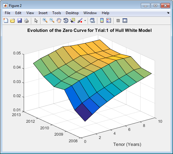
HW1FSimPaths = HW1F.simTermStructs(nPeriods,'NTRIALS',nTrials,...
    'DeltaTime',DeltaTime,'Tenor',Tenor,'antithetic',true);
trialIdx = 1;
figure
surf(Tenor,SimDates,HW1FSimPaths(:,:,trialIdx))
datetick y keepticks keeplimits
title(['Evolution of the Zero Curve for Trial:' num2str(trialIdx) ' of Hull White Model'])
xlabel('Tenor (Years)')
Price the European swaption.
DF = exp(bsxfun(@times,-HW1FSimPaths,repmat(Tenor',[nPeriods+1 1])));
SwapRate = (1 - DF(exRow,endCol,:))./sum(bsxfun(@times,1,DF(exRow,1:endCol,:)));
PayoffValue = 100*max(SwapRate-InstrumentStrike,0).*sum(bsxfun(@times,1,DF(exRow,1:endCol,:)));
RealizedDF = prod(exp(bsxfun(@times,-HW1FSimPaths(1:exRow,1,:),SimTimes(1:exRow))),1);
HW1F_SwaptionPrice = mean(RealizedDF.*PayoffValue)
HW1F_SwaptionPrice =

    2.1839
Simulate Interest-Rate Paths Using the Linear Gaussian Two-Factor Model
This example shows how to simulate interest-rate paths using
the Linear Gaussian two-factor model. Before beginning this example that uses a
LinearGaussian2F model, make sure that you have set up
the data as described in:
The Linear Gaussian two-factor model (called the G2++ by Brigo and Mercurio, see Interest-Rate Modeling Using Monte Carlo Simulation) is also a short rate model, but involves two factors. Specifically:
where is a two-dimensional Brownian motion with correlation ρ, and ϕ is a function chosen to match the initial zero curve.
The function swaptionbylg2f is used to compute analytic
values of the swaption price for model parameters, and therefore can be used to
calibrate the model. Calibration consists of minimizing the difference between
the observed market prices (computed above using the Black's implied swaption
volatility matrix, see Compute the Black Model and the Swaption Volatility Matrix) and the model’s
predicted prices.
In this example, the approach is similar to Simulate Interest-Rate Paths Using the Hull-White One-Factor Model
and the Optimization Toolbox function lsqnonlin is used to minimize the
difference between the observed swaption prices and the predicted swaption
prices. However, other approaches (for example, simulated annealing) may also be
appropriate. Starting parameters and constraints for a,
b, η, ρ, and
σ are set in the variables x0,
lb, and ub; these could also be varied
depending upon the particular calibration approach.
Calibrate the set of parameters that minimize the difference between the
observed and predicted values using swaptionbylg2f and
lsqnonlin.
G2PPobjfun = @(x) SwaptionBlackPrices(relidx) - swaptionbylg2f(irdc,x(1),x(2),x(3),x(4),x(5),SwaptionStrike(relidx),...
    EurExDatesFull(relidx),EurMatFull(relidx),'Reset',1);

options = optimset('disp','iter','MaxFunEvals',1000,'TolFun',1e-5);
x0 = [.2 .1 .02 .01 -.5];
lb = [0 0 0 0 -1];
ub = [1 1 1 1 1];
LG2Fparams = lsqnonlin(G2PPobjfun,x0,lb,ub,options)
                                         Norm of      First-order
 Iteration  Func-count     f(x)          step          optimality
     0          6         12.3547                          67.6
     1         12         1.37984      0.0979743           8.59
     2         18         1.37984       0.112847           8.59
     3         24        0.445202      0.0282118           1.31
     4         30        0.236746      0.0564236           3.02
     5         36        0.134678      0.0843366           7.78
     6         42       0.0398816       0.015084           6.34
     7         48       0.0287731       0.038967          0.732
     8         54       0.0273025       0.112847          0.881
     9         60       0.0241689       0.213033           1.06
    10         66       0.0241689       0.125602           1.06
    11         72       0.0239103      0.0314005           9.78
    12         78       0.0234246      0.0286685           1.21
    13         84       0.0234246      0.0491135           1.21
    14         90        0.023304      0.0122784           1.67
    15         96       0.0231931      0.0245568           5.92
    16        102       0.0230898     0.00785421          0.434
    17        108       0.0230898      0.0245568          0.434
    18        114        0.023083     0.00613919          0.255

Local minimum possible.

lsqnonlin stopped because the final change in the sum of squares relative to
its initial value is less than the selected value of the function tolerance.

LG2Fparams =

    0.5752    0.1181    0.0146    0.0119   -0.7895
Create the G2PP object using LinearGaussian2F and use
Monte Carlo simulation to generate the interest-rate paths with
LinearGaussian2F.simTermStructs.
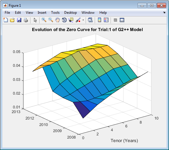
LG2f_a = LG2Fparams(1);
LG2f_b = LG2Fparams(2);
LG2f_sigma = LG2Fparams(3);
LG2f_eta = LG2Fparams(4);
LG2f_rho = LG2Fparams(5);

G2PP = LinearGaussian2F(RateSpec,LG2f_a,LG2f_b,LG2f_sigma,LG2f_eta,LG2f_rho);

G2PPSimPaths = G2PP.simTermStructs(nPeriods,'NTRIALS',nTrials,...
    'DeltaTime',DeltaTime,'Tenor',Tenor,'antithetic',true);

trialIdx = 1;
figure
surf(Tenor,SimDates,G2PPSimPaths(:,:,trialIdx))
datetick y keepticks keeplimits
title(['Evolution of the Zero Curve for Trial:' num2str(trialIdx) ' of G2++ Model'])
xlabel('Tenor (Years)')
Price the European swaption.
DF = exp(bsxfun(@times,-G2PPSimPaths,repmat(Tenor',[nPeriods+1 1])));
SwapRate = (1 - DF(exRow,endCol,:))./sum(bsxfun(@times,1,DF(exRow,1:endCol,:)));
PayoffValue = 100*max(SwapRate-InstrumentStrike,0).*sum(bsxfun(@times,1,DF(exRow,1:endCol,:)));
RealizedDF = prod(exp(bsxfun(@times,-G2PPSimPaths(1:exRow,1,:),SimTimes(1:exRow))),1);
G2PP_SwaptionPrice = mean(RealizedDF.*PayoffValue)
G2PP_SwaptionPrice =

    2.0988
Simulate Interest-Rate Paths Using the LIBOR Market Model
This example shows how to simulate interest-rate paths using
the LIBOR market model. Before beginning this example that uses a
LiborMarketModel, make sure that you have set up the data
as described in:
The LIBOR Market Model (LMM) differs from short rate models in that it evolves a set of discrete forward rates. Specifically, the lognormal LMM specifies the following diffusion equation for each forward rate
where:
W is an N-dimensional geometric Brownian motion with
The LMM relates the drifts of the forward rates based on no-arbitrage arguments. Specifically, under the Spot LIBOR measure, the drifts are expressed as
where:
is the time fraction associated with the ith forward rate
q(t) is an index defined by the relation
and the Spot LIBOR numeraire is defined as
The choice with the LMM is how to model volatility and correlation and how to estimate the parameters of these models for volatility and correlation. In practice, you may use a combination of historical data (for example, observed correlation between forward rates) and current market data. For this example, only swaption data is used. Further, many different parameterizations of the volatility and correlation exist. For this example, two relatively straightforward parameterizations are used.
One of the most popular functional forms in the literature for volatility is:
where ϕ adjusts the curve to match the
volatility for the i th forward rate. For this example, all
of the ϕ’s are taken to be 1. For the
correlation, the following functional form is used:
Once the functional forms have been specified, these parameters must be estimated using market data. One useful approximation, initially developed by Rebonato, is the following, which relates the Black volatility for a European swaption, given a set of volatility functions and a correlation matrix
where:
This calculation is done using the function
blackvolbyrebonato to compute analytic values of the
swaption price for model parameters, and therefore, is then used to calibrate
the model. Calibration consists of minimizing the difference between the
observed implied swaption Black volatilities and the predicted Black
volatilities.
In this example, the approach is similar to Simulate Interest-Rate Paths Using the Hull-White One-Factor Model
and Simulate Interest-Rate Paths Using the Linear Gaussian Two-Factor Model where the Optimization Toolbox function lsqnonlin is used to minimize the
difference between the observed swaption prices and the predicted swaption
prices. However, other approaches (for example, simulated annealing) may also be
appropriate. Starting parameters and constraints for a,
b, d, and β are set
in the variables x0, lb, and
ub; these could also be varied depending upon the
particular calibration approach.
Calibrate the set of parameters that minimize the difference between the
observed and predicted values using blackvolbyrebonato and
lsqnonlin.
nRates = 10;

CorrFunc = @(i,j,Beta) exp(-Beta*abs(i-j));

objfun = @(x) SwaptionBlackVol(relidx) - blackvolbyrebonato(RateSpec,...
    repmat({@(t) ones(size(t)).*(x(1)*t + x(2)).*exp(-x(3)*t) + x(4)},nRates-1,1),...
    CorrFunc(meshgrid(1:nRates-1)',meshgrid(1:nRates-1),x(5)),...
    EurExDatesFull(relidx),EurMatFull(relidx),'Period',1);

options = optimset('disp','iter','MaxFunEvals',1000,'TolFun',1e-5);

x0 = [.2 .05 1 .05 .2];
lb = [0 0 .5 0 .01];
ub = [1 1 2 .3 1];
LMMparams = lsqnonlin(objfun,x0,lb,ub,options)
                                        Norm of      First-order
 Iteration  Func-count     f(x)          step          optimality
     0          6        0.156251                         0.483
     1         12      0.00870177       0.188164         0.0339
     2         18      0.00463441       0.165527        0.00095
     3         24      0.00331055       0.351017         0.0154
     4         30      0.00294775      0.0892617       7.47e-05
     5         36      0.00281565       0.385779        0.00917
     6         42      0.00278988      0.0145632       4.15e-05
     7         48      0.00278522       0.115042        0.00116
Local minimum possible.

lsqnonlin stopped because the final change in the sum of squares relative to
its initial value is less than the selected value of the function tolerance.

LMMparams =

    0.0781    0.1656    0.5121    0.0617    0.0100
Calculate VolFunc for the LMM
object.
a = LMMparams(1);
b = LMMparams(2);
c = LMMparams(3);
d = LMMparams(4);

Beta = LMMparams(5);

VolFunc = repmat({@(t) ones(size(t)).*(a*t + b).*exp(-c*t) + d},nRates-1,1);
Plot the volatility function.
figure
fplot(VolFunc{1},[0 20])
title('Volatility Function')

CorrelationMatrix = CorrFunc(meshgrid(1:nRates-1)',meshgrid(1:nRates-1),Beta);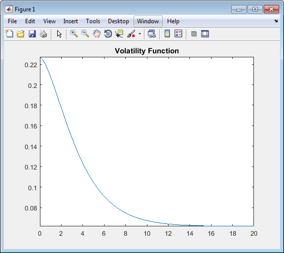
Inspect the correlation matrix.
disp('Correlation Matrix')
fprintf([repmat('%1.3f ',1,length(CorrelationMatrix)) ' \n'],CorrelationMatrix)
Correlation Matrix
1.000 0.990 0.980 0.970 0.961 0.951 0.942 0.932 0.923
0.990 1.000 0.990 0.980 0.970 0.961 0.951 0.942 0.932
0.980 0.990 1.000 0.990 0.980 0.970 0.961 0.951 0.942
0.970 0.980 0.990 1.000 0.990 0.980 0.970 0.961 0.951
0.961 0.970 0.980 0.990 1.000 0.990 0.980 0.970 0.961
0.951 0.961 0.970 0.980 0.990 1.000 0.990 0.980 0.970
0.942 0.951 0.961 0.970 0.980 0.990 1.000 0.990 0.980
0.932 0.942 0.951 0.961 0.970 0.980 0.990 1.000 0.990
0.923 0.932 0.942 0.951 0.961 0.970 0.980 0.990 1.000
Create the LMM object using LiborMarketModel and use
Monte Carlo simulation to generate the interest-rate paths with
LiborMarketModel.simTermStructs.
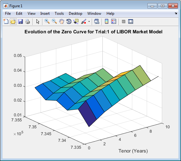
LMM = LiborMarketModel(irdc,VolFunc,CorrelationMatrix,'Period',1);

[LMMZeroRates, ForwardRates] = LMM.simTermStructs(nPeriods,'nTrials',nTrials);

trialIdx = 1;
figure
tmpPlotData = LMMZeroRates(:,:,trialIdx);
tmpPlotData(tmpPlotData == 0) = NaN;
surf(Tenor,SimDates,tmpPlotData)
title(['Evolution of the Zero Curve for Trial:' num2str(trialIdx) ' of LIBOR Market Model'])
xlabel('Tenor (Years)')
Price the European swaption.
DF = exp(bsxfun(@times,-LMMZeroRates,repmat(Tenor',[nPeriods+1 1])));
SwapRate = (1 - DF(exRow,endCol,:))./sum(bsxfun(@times,1,DF(exRow,1:endCol,:)));
PayoffValue = 100*max(SwapRate-InstrumentStrike,0).*sum(bsxfun(@times,1,DF(exRow,1:endCol,:)));
RealizedDF = prod(exp(bsxfun(@times,-LMMZeroRates(2:exRow+1,1,:),SimTimes(1:exRow))),1);
LMM_SwaptionPrice = mean(RealizedDF.*PayoffValue)
LMM_SwaptionPrice =

    1.9915
Compare Interest-Rate Modeling Results
This example shows how to compare the results for pricing a European swaption with different interest-rate models.
Compare the results for pricing a European swaption with interest-rate models using Monte Carlo simulation.
disp(' ')
fprintf('     # of Monte Carlo Trials: %8d\n'    , nTrials)
fprintf('     # of Time Periods/Trial: %8d\n\n'  , nPeriods)
fprintf('HW1F European Swaption Price: %8.4f\n', HW1F_SwaptionPrice)
fprintf('LG2F Europesn Swaption Price: %8.4f\n', G2PP_SwaptionPrice)
fprintf(' LMM European Swaption Price: %8.4f\n', LMM_SwaptionPrice)
 # of Monte Carlo Trials:     1000
     # of Time Periods/Trial:        5

HW1F European Swaption Price:   2.1839
LG2F Europesn Swaption Price:   2.0988
 LMM European Swaption Price:   1.9915
References
Brigo, D. and F. Mercurio. Interest Rate Models - Theory and Practice with Smile, Inflation and Credit. Springer Finance, 2006.
Andersen, L. and V. Piterbarg. Interest Rate Modeling. Atlantic Financial Press. 2010.
Hull, J. Options, Futures, and Other Derivatives. Springer Finance, 2003.
Glasserman, P. Monte Carlo Methods in Financial Engineering. Prentice Hall, 2008.
Rebonato, R., K. McKay, and R. White. The Sabr/Libor Market Model: Pricing, Calibration and Hedging for Complex Interest-Rate Derivatives. John Wiley & Sons, 2010.
See Also
HullWhite1F | LinearGaussian2F | LiborMarketModel | simTermStructs | simTermStructs | simTermStructs | capbylg2f | floorbylg2f | swaptionbylg2f | swaptionbyhw | blackvolbyrebonato | lsqnonlin