Pricing Bermudan Swaptions with Monte Carlo Simulation
This example shows how to price Bermudan swaptions using interest-rate models in Financial Instruments Toolbox™. Specifically, a Hull-White one factor model, a Linear Gaussian two-factor model, and a LIBOR Market Model are calibrated to market data and then used to generate interest-rate paths using Monte Carlo simulation.
Zero Curve
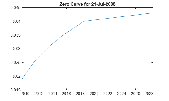
In this example, the ZeroRates for a zero curve is hard-coded. You can also create a zero curve by bootstrapping the zero curve from market data (for example, deposits, futures/forwards, and swaps). The hard-coded data for the zero curve is defined as:
Settle = datetime(2008,7,21);

% Zero Curve
CurveDates = daysadd(Settle,360*([1 3 5 7 10 20]),1);
ZeroRates = [1.9 2.6 3.1 3.5 4 4.3]'/100;

plot(CurveDates,ZeroRates)
title(['Zero Curve for ' datestr(Settle)]);
RateSpec = intenvset('Rates',ZeroRates,'EndDates',CurveDates,'StartDate',Settle);
Define Swaption Parameters
For this example, you compute the price of a 10-no-call-1 Bermudan swaption.
BermudanExerciseDates = daysadd(Settle,360*(1:9),1);
BermudanMaturity = datetime(2018,7,21);
BermudanStrike = .045;
Black's Model and the Swaption Volatility Matrix
Black's model is often used to price and quote European exercise interest-rate options, that is, caps, floors, and swaptions. In the case of swaptions, Black's model is used to imply a volatility given the current observed market price. The following matrix shows the Black implied volatility for a range of swaption exercise dates (columns) and underlying swap maturities (rows).
SwaptionBlackVol = [22 21 19 17 15 13 12
    21 19 17 16 15 13 11
    20 18 16 15 14 12 11
    19 17 15 14 13 12 10
    18 16 14 13 12 11 10
    15 14 13 12 12 11 10
    13 13 12 11 11 10 9]/100;
ExerciseDates = [1:5 7 10];
Tenors = [1:5 7 10];

EurExDatesFull = repmat(daysadd(Settle,ExerciseDates*360,1)',...
    length(Tenors),1);
EurMatFull = reshape(daysadd(EurExDatesFull,...
    repmat(360*Tenors,1,length(ExerciseDates)),1),size(EurExDatesFull));
Selecting the Calibration Instruments
Selecting the instruments to calibrate the model to is one of the tasks in calibration. For Bermudan swaptions, it is typical to calibrate to European swaptions that are co-terminal with the Bermudan swaption that you want to price. In this case, all swaptions having an underlying tenor that matures before the maturity of the swaption to be priced are used in the calibration.
% Find the swaptions that expire on or before the maturity date of the
% sample swaption
relidx = find(EurMatFull <= BermudanMaturity);
Compute Swaption Prices Using Black's Model
Swaption prices are computed using Black's Model. You can then use the swaption prices to compare the model's predicted values. To compute the swaption prices using Black's model:
% Compute Swaption Prices using Black's model
SwaptionBlackPrices = zeros(size(SwaptionBlackVol));
SwaptionStrike = zeros(size(SwaptionBlackVol));

for iSwaption=1:length(ExerciseDates)
    for iTenor=1:length(Tenors)
        [~,SwaptionStrike(iTenor,iSwaption)] = swapbyzero(RateSpec,[NaN 0], Settle, EurMatFull(iTenor,iSwaption),...
            'StartDate',EurExDatesFull(iTenor,iSwaption),'LegReset',[1 1]);
        SwaptionBlackPrices(iTenor,iSwaption) = swaptionbyblk(RateSpec, 'call', SwaptionStrike(iTenor,iSwaption),Settle, ...
            EurExDatesFull(iTenor,iSwaption), EurMatFull(iTenor,iSwaption), SwaptionBlackVol(iTenor,iSwaption));
    end
end
Simulation Parameters
The following parameters are used where each exercise date is a simulation date.
nPeriods = 9;
DeltaTime = 1;
nTrials = 1000;

Tenor = (1:10)';

SimDates = daysadd(Settle,360*DeltaTime*(0:nPeriods),1);
SimTimes = diff(yearfrac(SimDates(1),SimDates));
Hull White 1 Factor Model
The Hull-White one-factor model describes the evolution of the short rate and is specified by the following:
The Hull-White model is calibrated using the function swaptionbyhw, which constructs a trinomial tree to price the swaptions. Calibration consists of minimizing the difference between the observed market prices (computed above using the Black's implied swaption volatility matrix) and the model's predicted prices.
This example uses the Optimization Toolbox™ function lsqnonlin to find the parameter set that minimizes the difference between the observed and predicted values. However, other approaches (for example, simulated annealing) may be appropriate. Starting parameters and constraints for and are set in the variables x0 , lb, and ub; these could also be varied depending upon the particular calibration approach.
warnId = 'fininst:swaptionbyirtree:IgnoredSettle';
warnStruct = warning('off',warnId); % Turn warning off

TimeSpec = hwtimespec(Settle,daysadd(Settle,360*(1:11),1), 2);
HW1Fobjfun = @(x) SwaptionBlackPrices(relidx) - ...
    swaptionbyhw(hwtree(hwvolspec(Settle,datetime(2015,8,11),x(2),datetime(2015,8,11),x(1)), RateSpec, TimeSpec), 'call', SwaptionStrike(relidx),...
    EurExDatesFull(relidx), 0, EurExDatesFull(relidx), EurMatFull(relidx));
options = optimset('disp','iter','MaxFunEvals',1000,'TolFun',1e-5);

% Find the parameters that minimize the difference between the observed and
% predicted prices
x0 = [.1 .01];
lb = [0 0];
ub = [1 1];

HW1Fparams = lsqnonlin(HW1Fobjfun,x0,lb,ub,options);
                                            Norm of      First-order
 Iteration  Func-count      Resnorm            step       optimality
     0          3          0.953772                             20.5
     1          6          0.142828       0.0169199             1.53
     2          9          0.123022       0.0146705             2.31
     3         12          0.122222       0.0154099            0.482
     4         15          0.122217      0.00131297           0.0041

Local minimum possible.

lsqnonlin stopped because the final change in the sum of squares relative to
its initial value is less than the value of the function tolerance.

<stopping criteria details>
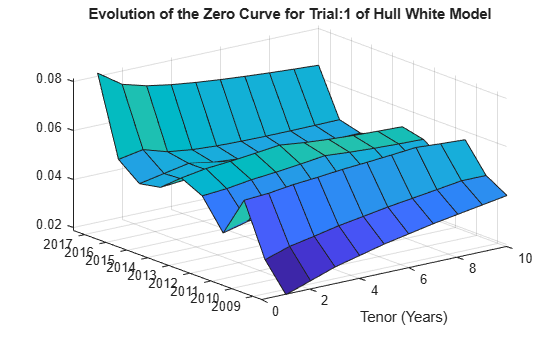
warning(warnStruct); % Turn warnings on

HW_alpha = HW1Fparams(1);
HW_sigma = HW1Fparams(2);

% Construct the HullWhite1F model using the HullWhite1F constructor.
HW1F = HullWhite1F(RateSpec,HW_alpha,HW_sigma);

% Use Monte Carlo simulation to generate the interest-rate paths with
% HullWhite1F.simTermStructs.
HW1FSimPaths = HW1F.simTermStructs(nPeriods,'NTRIALS',nTrials,...
    'DeltaTime',DeltaTime,'Tenor',Tenor,'antithetic',true);

% Examine one simulation
trialIdx = 1;
figure
surf(Tenor,SimDates,HW1FSimPaths(:,:,trialIdx))
ytickformat; % y keepticks keeplimits
title(['Evolution of the Zero Curve for Trial:' num2str(trialIdx) ' of Hull White Model'])
xlabel('Tenor (Years)')
% Price the swaption using the helper function hBermudanSwaption
HW1FBermPrice = hBermudanSwaption(HW1FSimPaths,SimDates,Tenor,BermudanStrike,...
    BermudanExerciseDates,BermudanMaturity);
Linear Gaussian 2 Factor Model
The Linear Gaussian two-factor model (called the G2++ by Brigo and Mercurio) is also a short rate model, but involves two factors. Specifically:
where is a two-dimensional Brownian motion with correlation
and is a function chosen to match the initial zero curve.
You can use the function swaptionbylg2f to compute analytic values of the swaption price for model parameters and to calibrate the model. Calibration consists of minimizing the difference between the observed market prices and the model's predicted prices.
% Calibrate the set of parameters that minimize the difference between the
% observed and predicted values using swaptionbylg2f and lsqnonlin.
G2PPobjfun = @(x) SwaptionBlackPrices(relidx) - ...
    swaptionbylg2f(RateSpec,x(1),x(2),x(3),x(4),x(5),SwaptionStrike(relidx),...
    EurExDatesFull(relidx),EurMatFull(relidx),'Reset',1);
x0 = [.2 .1 .02 .01 -.5];
lb = [0 0 0 0 -1];
ub = [1 1 1 1 1];
LG2Fparams = lsqnonlin(G2PPobjfun,x0,lb,ub,options);
                                            Norm of      First-order
 Iteration  Func-count      Resnorm            step       optimality
     0          6           11.9838                             66.5
     1         12           1.35076       0.0967223             8.47
     2         18           1.35076        0.111744             8.47
     3         24          0.439341       0.0279361             1.29
     4         30          0.237917       0.0558721             3.49
     5         36          0.126732       0.0836847             7.51
     6         42         0.0395759       0.0137736             7.43
     7         48         0.0265828       0.0355773            0.787
     8         54         0.0252764        0.111744              0.5
     9         60         0.0228936        0.196793            0.338
    10         66         0.0222739        0.106677           0.0946
    11         72         0.0221799       0.0380096            0.912
    12         78         0.0221726       0.0163292             1.37

Local minimum possible.

lsqnonlin stopped because the final change in the sum of squares relative to
its initial value is less than the value of the function tolerance.

<stopping criteria details>
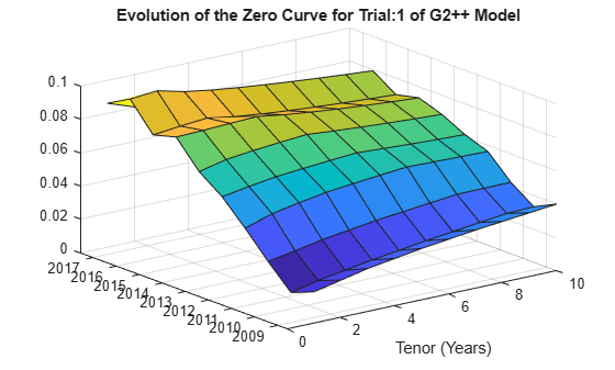
LG2f_a = LG2Fparams(1);
LG2f_b = LG2Fparams(2);
LG2f_sigma = LG2Fparams(3);
LG2f_eta = LG2Fparams(4);
LG2f_rho = LG2Fparams(5);

% Create the G2PP object and use Monte Carlo simulation to generate the
% interest-rate paths with LinearGaussian2F.simTermStructs.
G2PP = LinearGaussian2F(RateSpec,LG2f_a,LG2f_b,LG2f_sigma,LG2f_eta,LG2f_rho);

G2PPSimPaths = G2PP.simTermStructs(nPeriods,'NTRIALS',nTrials,...
    'DeltaTime',DeltaTime,'Tenor',Tenor,'antithetic',true);

% Examine one simulation
trialIdx = 1;
figure
surf(Tenor,SimDates,G2PPSimPaths(:,:,trialIdx))
ytickformat; % y keepticks keeplimits
title(['Evolution of the Zero Curve for Trial:' num2str(trialIdx) ' of G2++ Model'])
xlabel('Tenor (Years)')
% Price the swaption using the helper function hBermudanSwaption
LG2FBermPrice = hBermudanSwaption(G2PPSimPaths,SimDates,Tenor,BermudanStrike,BermudanExerciseDates,BermudanMaturity);
LIBOR Market Model
The LIBOR Market Model (LMM) differs from short rate models in that it evolves a set of discrete forward rates. Specifically, the lognormal LMM specifies the following diffusion equation for each forward rate
where
is the volatility function for each rate and is an N dimensional geometric Brownian motion with:
The LMM relates the drifts of the forward rates based on no-arbitrage arguments.
The choice with the LMM is how to model volatility and correlation and how to estimate the parameters of these models for volatility and correlation. In practice, you might use a combination of historical data (for example, observed correlation between forward rates) and current market data. For this example, only swaption data is used. Furthermore, many different parameterizations of the volatility and correlation exist. This example uses two relatively straightforward parameterizations.
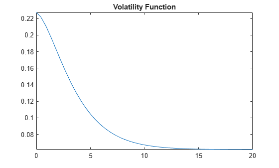
One of the most popular functional forms in the literature for volatility is:
where adjusts the curve to match the volatility for the forward rate. For this example, all of the Phi's will be taken to be 1.
For the correlation, the following functional form is used:
Once the functional forms are specified, the parameters need to be estimated using market data. One useful approximation, initially developed by Rebonato, is the following, which computes the Black volatility for a European swaption, given a LMM with a set of volatility functions and a correlation matrix.
where
This calculation is done using blackvolbyrebonato to compute analytic values of the swaption price for model parameters and also to calibrate the model. Calibration consists of minimizing the difference between the observed implied swaption Black volatilities and the predicted Black volatilities.
nRates = 10;

CorrFunc = @(i,j,Beta) exp(-Beta*abs(i-j));

objfun = @(x) SwaptionBlackVol(relidx) - blackvolbyrebonato(RateSpec,...
    repmat({@(t) ones(size(t)).*(x(1)*t + x(2)).*exp(-x(3)*t) + x(4)},nRates-1,1),...
    CorrFunc(meshgrid(1:nRates-1)',meshgrid(1:nRates-1),x(5)),...
    EurExDatesFull(relidx),EurMatFull(relidx),'Period',1);

x0 = [.2 .05 1 .05 .2];
lb = [0 0 .5 0 .01];
ub = [1 1 2 .3 1];
LMMparams = lsqnonlin(objfun,x0,lb,ub,options);
                                            Norm of      First-order
 Iteration  Func-count      Resnorm            step       optimality
     0          6          0.156251                            0.483
     1         12        0.00870177        0.188164           0.0339
     2         18        0.00463441        0.165527          0.00095
     3         24        0.00331055        0.351017           0.0154
     4         30        0.00294775       0.0892616         7.47e-05
     5         36        0.00281565        0.385779          0.00917
     6         42        0.00278988       0.0145632         4.15e-05
     7         48        0.00278522        0.115042          0.00116

Local minimum possible.

lsqnonlin stopped because the final change in the sum of squares relative to
its initial value is less than the value of the function tolerance.

<stopping criteria details>
% Calculate VolFunc for the LMM object.
a = LMMparams(1);
b = LMMparams(2);
c = LMMparams(3);
d = LMMparams(4);

Beta = LMMparams(5);

VolFunc = repmat({@(t) ones(size(t)).*(a*t + b).*exp(-c*t) + d},nRates-1,1);

% Plot the volatility function
figure
fplot(VolFunc{1},[0 20])
title('Volatility Function')
% Inspect the correlation matrix
CorrelationMatrix = CorrFunc(meshgrid(1:nRates-1)',meshgrid(1:nRates-1),Beta);
displayCorrelationMatrix(CorrelationMatrix);
Correlation Matrix 1.000 0.990 0.980 0.970 0.961 0.951 0.942 0.932 0.923 0.990 1.000 0.990 0.980 0.970 0.961 0.951 0.942 0.932 0.980 0.990 1.000 0.990 0.980 0.970 0.961 0.951 0.942 0.970 0.980 0.990 1.000 0.990 0.980 0.970 0.961 0.951 0.961 0.970 0.980 0.990 1.000 0.990 0.980 0.970 0.961 0.951 0.961 0.970 0.980 0.990 1.000 0.990 0.980 0.970 0.942 0.951 0.961 0.970 0.980 0.990 1.000 0.990 0.980 0.932 0.942 0.951 0.961 0.970 0.980 0.990 1.000 0.990 0.923 0.932 0.942 0.951 0.961 0.970 0.980 0.990 1.000
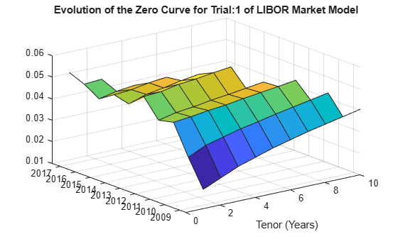
% Create the LMM object and use Monte Carlo simulation to generate the
% interest-rate paths with LiborMarketModel.simTermStructs.
LMM = LiborMarketModel(RateSpec,VolFunc,CorrelationMatrix,'Period',1);

[LMMZeroRates, ForwardRates] = LMM.simTermStructs(nPeriods,'nTrials',nTrials);

% Examine one simulation
trialIdx = 1;
figure
tmpPlotData = LMMZeroRates(:,:,trialIdx);
tmpPlotData(tmpPlotData == 0) = NaN;
surf(Tenor,SimDates,tmpPlotData)
title(['Evolution of the Zero Curve for Trial:' num2str(trialIdx) ' of LIBOR Market Model'])
xlabel('Tenor (Years)')
% Price the swaption using the helper function hBermudanSwaption
LMMTenor = 1:10;
LMMBermPrice = hBermudanSwaption(LMMZeroRates,SimDates,LMMTenor,.045,BermudanExerciseDates,BermudanMaturity);
Results
displayResults(nTrials, nPeriods, HW1FBermPrice, LG2FBermPrice, LMMBermPrice);
     # of Monte Carlo Trials:     1000
     # of Time Periods/Trial:        9

HW1F Bermudan Swaption Price:   3.7577
LG2F Bermudan Swaption Price:   3.5576
 LMM Bermudan Swaption Price:   3.4911
Bibliography
This example is based on the following books, papers and journal articles:
Andersen, L. and V. Piterbarg. Interest Rate Modeling. Atlantic Financial Press, 2010.
Brigo, D. and F. Mercurio. Interest Rate Models - Theory and Practice with Smile, Inflation and Credit. Springer Verlag, 2007.
Glasserman, P. Monte Carlo Methods in Financial Engineering. Springer, 2003.
Hull, J. Options, Futures, and Other Derivatives. Prentice Hall, 2008.
Rebonato, R., K. McKay, and R. White. The Sabr/Libor Market Model: Pricing, Calibration and Hedging for Complex Interest-Rate Derivatives. John Wiley & Sons, 2010.
Local Functions
function displayCorrelationMatrix(CorrelationMatrix)
fprintf('Correlation Matrix\n');
fprintf([repmat('%1.3f ',1,length(CorrelationMatrix)) ' \n'],CorrelationMatrix);
end

function displayResults(nTrials, nPeriods, HW1FBermPrice, LG2FBermPrice, LMMBermPrice)
fprintf('     # of Monte Carlo Trials: %8d\n'    , nTrials);
fprintf('     # of Time Periods/Trial: %8d\n\n'  , nPeriods);
fprintf('HW1F Bermudan Swaption Price: %8.4f\n', HW1FBermPrice);
fprintf('LG2F Bermudan Swaption Price: %8.4f\n', LG2FBermPrice);
fprintf(' LMM Bermudan Swaption Price: %8.4f\n', LMMBermPrice);
end
See Also
capbyblk | floorbyblk | swaptionbyblk | blackvolbysabr | optsensbysabr | agencyoas | agencyprice | bndfutimprepo | bndfutprice | convfactor | tfutbyprice | tfutbyyield | tfutimprepo | tfutpricebyrepo | tfutyieldbyrepo | capbylg2f | floorbylg2f | swaptionbylg2f | blackvolbyrebonato | hwcalbycap | hwcalbyfloor
Topics
- Calibrate the SABR Model
- Price a Swaption Using the SABR Model
- Computing the Agency OAS for Bonds
- Analysis of Bond Futures
- Managing Interest-Rate Risk with Bond Futures
- Fitting the Diebold Li Model
- Price Swaptions with Interest-Rate Models Using Simulation
- Managing Present Value with Bond Futures
- Supported Interest-Rate Instrument Functions
- Supported Equity Derivative Functions
- Supported Energy Derivative Functions
- Mapping Financial Instruments Toolbox Functions for Interest-Rate Instrument Objects