HullWhite1F
Create Hull-White one-factor model
Description
The Hull-White one-factor model is specified using the zero curve, alpha, and sigma parameters.
Specifically, the HullWhite1F model is defined using the following equation:
where
dr is the change in the short-term interest rate over a small interval.
r is the short-term interest rate.
Θ(t) is a function of time determining the average direction in which r moves, chosen such that movements in r are consistent with today's zero coupon yield curve.
α is the mean reversion rate.
dt is a small change in time.
σ is the annual standard deviation of the short rate.
W is the Brownian motion.
Creation
Description
HW1F = HullWhite1F(ZeroCurve,Alpha,Sigma)HullWhite1F (HW1F) object using the
required arguments to set the Properties.
Input Arguments
Output Arguments
Properties
Object Functions
simTermStructs | Simulate term structures for Hull-White one-factor model |
Examples
Create a Hull-White one-factor model using an IRDataCurve.
Settle = datetime(2007,12,15);
CurveTimes = [1:5 7 10 20]';
ZeroRates = [.01 .018 .024 .029 .033 .034 .035 .034]';
CurveDates = daysadd(Settle,360*CurveTimes,1);

irdc = IRDataCurve('Zero',Settle,CurveDates,ZeroRates);

alpha = .1;
sigma = .01;

HW1F = HullWhite1F(irdc,alpha,sigma)
HW1F =
HullWhite1F with properties:
ZeroCurve: [1×1 IRDataCurve]
Alpha: @(t,V)inAlpha
Sigma: @(t,V)inSigma
Use the simTermStructs method with the HullWhite1F model to simulate term structures.
SimPaths = simTermStructs(HW1F, 10,'nTrials',100);Create a Hull-White one-factor model using a RateSpec.
Settle = datetime(2007,12,15); CurveTimes = [1:5 7 10 20]'; ZeroRates = [.01 .018 .024 .029 .033 .034 .035 .034]'; CurveDates = daysadd(Settle,360*CurveTimes,1); RateSpec = intenvset('Rates',ZeroRates,'EndDates',CurveDates,'StartDate',Settle); alpha = .1; sigma = .01; HW1F = HullWhite1F(RateSpec,alpha,sigma)
HW1F =
  HullWhite1F with properties:

    ZeroCurve: [1×1 IRDataCurve]
        Alpha: @(t,V)inAlpha
        Sigma: @(t,V)inSigma
Use the simTermStructs method with the HullWhite1F model to simulate term structures.
SimPaths = simTermStructs(HW1F, 10,'nTrials',100);Define the zero curve data.
Settle = datetime(2016,4,4); ZeroTimes = [3/12 6/12 1 5 7 10 20 30]'; ZeroRates = [0.033 0.034 0.035 0.040 0.042 0.044 0.048 0.0475]'; ZeroDates = datemnth(Settle,ZeroTimes*12); RateSpec = intenvset('StartDates', Settle,'EndDates', ZeroDates, 'Rates', ZeroRates)
RateSpec = struct with fields:
FinObj: 'RateSpec'
Compounding: 2
Disc: [8×1 double]
Rates: [8×1 double]
EndTimes: [8×1 double]
StartTimes: [8×1 double]
EndDates: [8×1 double]
StartDates: 736424
ValuationDate: 736424
Basis: 0
EndMonthRule: 1
Define the bond parameters.
Maturity = datemnth(Settle,12*5); CouponRate = 0;
Define the Hull-White parameters.
alpha = .1; sigma = .01; HW1F = HullWhite1F(RateSpec,alpha,sigma)
HW1F =
  HullWhite1F with properties:

    ZeroCurve: [1×1 IRDataCurve]
        Alpha: @(t,V)inAlpha
        Sigma: @(t,V)inSigma
Define the simulation parameters.
nTrials = 100; nPeriods = 12*5; deltaTime = 1/12; SimZeroCurvePaths = simTermStructs(HW1F, nPeriods,'nTrials',nTrials,'deltaTime',deltaTime); SimDates = datemnth(Settle,1:nPeriods);
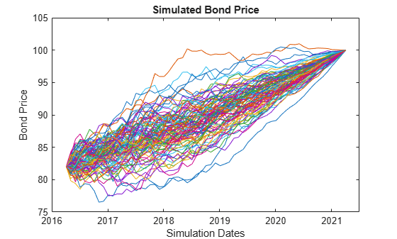
Preallocate and initialize for the simulation.
SimBondPrice = zeros(nPeriods+1,nTrials); SimBondPrice(1,:,:) = bondbyzero(RateSpec,CouponRate,Settle,Maturity); SimBondPrice(end,:,:) = 100;
Compute the bond values for each simulation date and path, note that you can vectorize over the trial dimension.
for periodidx=1:nPeriods-1 simRateSpec = intenvset('StartDate',SimDates(periodidx),'EndDates',... datemnth(SimDates(periodidx),ZeroTimes*12),'Rates',squeeze(SimZeroCurvePaths(periodidx+1,:,:))); SimBondPrice(periodidx+1,:) = bondbyzero(simRateSpec,CouponRate,SimDates(periodidx),Maturity); end plot([Settle SimDates],SimBondPrice) ylabel('Bond Price') xlabel('Simulation Dates') title('Simulated Bond Price')
Define the zero curve data.
Settle = datetime(2016,4,4); ZeroTimes = [3/12 6/12 1 5 7 10 20 30]'; ZeroRates = [-0.01 -0.009 -0.0075 -0.003 -0.002 -0.001 0.002 0.0075]'; ZeroDates = datemnth(Settle,ZeroTimes*12); RateSpec = intenvset('StartDates', Settle,'EndDates', ZeroDates, 'Rates', ZeroRates)
RateSpec = struct with fields:
           FinObj: 'RateSpec'
      Compounding: 2
             Disc: [8×1 double]
            Rates: [8×1 double]
         EndTimes: [8×1 double]
       StartTimes: [8×1 double]
         EndDates: [8×1 double]
       StartDates: 736424
    ValuationDate: 736424
            Basis: 0
     EndMonthRule: 1
Define the bond parameters for the five bonds in the portfolio.
Maturity = datemnth(Settle,12*5); % All bonds have the same maturity CouponRate = [0.035;0.04;0.02;0.015;0.042]; % Different coupon rates for the bonds nBonds = length(CouponRate);
Define the Hull-White parameters.
alpha = .1;
sigma = .01;
HW1F = HullWhite1F(RateSpec,alpha,sigma)
HW1F =
  HullWhite1F with properties:

    ZeroCurve: [1×1 IRDataCurve]
        Alpha: @(t,V)inAlpha
        Sigma: @(t,V)inSigma
Define the simulation parameters.
nTrials = 1000;
nPeriods = 12*5;
deltaTime = 1/12;
SimZeroCurvePaths = simTermStructs(HW1F, nPeriods,'nTrials',nTrials,'deltaTime',deltaTime);
SimDates = datemnth(Settle,1:nPeriods);
Preallocate and initialize for the simulation.
SimBondPrice = zeros(nPeriods+1,nBonds,nTrials);
SimBondPrice(1,:,:) = repmat(bondbyzero(RateSpec,CouponRate,Settle,Maturity)',[1 1 nTrials]);
SimBondPrice(end,:,:) = 100;

[BondCF,BondCFDates,~,CFlowFlags] = cfamounts(CouponRate,Settle,Maturity);
BondCF(CFlowFlags == 4) = BondCF(CFlowFlags == 4) - 100;
SimBondCF = zeros(nPeriods+1,nBonds,nTrials);
Compute bond values for each simulation date and path. Note that you can vectorize over the trial dimension.
for periodidx=1:nPeriods
    if periodidx < nPeriods
        simRateSpec = intenvset('StartDate',SimDates(periodidx),'EndDates',...
            datemnth(SimDates(periodidx),ZeroTimes*12),'Rates',squeeze(SimZeroCurvePaths(periodidx+1,:,:)));
        SimBondPrice(periodidx+1,:,:) = bondbyzero(simRateSpec,CouponRate,SimDates(periodidx),Maturity);
    end

    simidx = SimDates(periodidx) == BondCFDates;
    SimCF = zeros(1,nBonds);
    SimCF(any(simidx,2)) = BondCF(simidx);
    ReinvestRate = 1 + SimZeroCurvePaths(periodidx+1,1,:);
    SimBondCF(periodidx+1,:,:) = bsxfun(@times,bsxfun(@plus,SimBondCF(periodidx,:,:),SimCF),ReinvestRate);
end
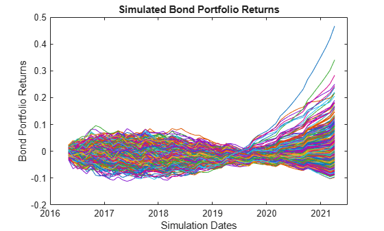
Compute the total return series.
TotalCF = SimBondPrice + SimBondCF;
Assume the bond portfolio is equally weighted and plot the simulated bond portfolio returns.
TotalCF = squeeze(sum(TotalCF,2));

TotRetSeries = bsxfun(@rdivide,TotalCF(2:end,:),TotalCF(1,:)) - 1;
plot(SimDates,TotRetSeries)
ylabel('Bond Portfolio Returns')
xlabel('Simulation Dates')
title('Simulated Bond Portfolio Returns')
More About
References
[1] Brigo, D. and F. Mercurio. Interest Rate Models - Theory and Practice. Springer Finance, 2006.
[2] Hull, J. Options, Futures, and Other Derivatives. Prentice-Hall, 2011.
Version History
Introduced in R2013a