SABRBraceGatarekMusiela
Create SABRBraceGatarekMusiela model object for
Cap, Floor, FixedBond,
FloatBond, FloatBondOption,
FixedBondOption, OptionEmbeddedFixedBond, or
OptionEmbeddedFloatBond instrument
Since R2021b
Description
Create and price a Cap, Floor,
FloatBond, FloatBondOption,
FixedBond, FixedBondOption,
OptionEmbeddedFixedBond, or
OptionEmbeddedFloatBond instrument object with a
SABRBraceGatarekMusiela model using this workflow:
Use
fininstrumentto create aCap,Floor,FixedBond,FloatBond,FloatBondOptionFixedBondOption,OptionEmbeddedFixedBond, orOptionEmbeddedFloatBondinstrument object.Use
finmodelto specify aSABRBraceGatarekMusielamodel object for theCap,Floor,FixedBond,FloatBond,FloatBondOption,FixedBondOption,OptionEmbeddedFixedBond, orOptionEmbeddedFloatBondinstrument object.Use
finpricerto specify anIRMonteCarlopricing method for aCap,Floor,FixedBond,FloatBond,FloatBondOption,FixedBondOption,OptionEmbeddedFixedBond, orOptionEmbeddedFloatBondinstrument object.
For more information on this workflow, see Get Started with Workflows Using Object-Based Framework for Pricing Financial Instruments.
For more information on the available pricing methods for a Cap,
Floor, FixedBond,
FloatBond, FloatBondOption,
FixedBondOption, OptionEmbeddedFixedBond, or
OptionEmbeddedFloatBond instrument, see Choose Instruments, Models, and Pricers.
Creation
Description
SABRBraceGatarekMusielaModelObj = finmodel(ModelType,Alpha=alpha_value,Beta=beta_value,VolatilityofVolatility=volatilityofvolatility_value,FwdFwdCorrelation=fwdfwdcorrelation_value,VolVolCorrelation=volvolcorrelation_value)SABRBraceGatarekMusiela model object
with null forward to volatility correlation by specifying
ModelType and the required name-value arguments
Alpha, Beta,
VolatilityofVolatility,
FwdFwdCorrelation, and
VolVolCorrelation to set properties
using name-value arguments. For example,
SABRBraceGatarekMusielaModelObj =
                            finmodel("SABRBraceGatarekMusiela",Alpha=Alpha,Beta=Beta,VolatilityofVolatility=VolVolFunc,FwdFwdCorrelation=FwdFwdCorrelation,
                            VolVolCorrelation=VolVolCorrelation)
creates a classic
SABRBraceGatarekMusiela model object with null
forward to volatility correlation.
SABRBraceGatarekMusielaModelObj = finmodel(___,Name=Value)SABRBraceGatarekMusiela model:
To create a classic
SABRBraceGatarekMusielamodel object, use theFwdVolCorrelationname-value pair argument:SABRBraceGatarekMusielaModelObj = finmodel("SABRBraceGatarekMusiela",Alpha=Alpha,Beta=Beta,VolatilityofVolatility=VolVolFunc,FwdFwdCorrelation=FwdFwdCorrelation,VolVolCorrelation=VolVolCorrelation,FwdVolCorrelation=FwdVolCorrelation)To create a classic
SABRBraceGatarekMusielamodel object in Rebonato parametric form with null forward-to-volatility correlation, use theVolatilityname-value pair argument:SABRBraceGatarekMusielaModelObj = finmodel("SABRBraceGatarekMusiela",Alpha=Alpha,Beta=Beta,VolatilityofVolatility=VolVolFunc,Volatility=VolFunc,FwdFwdCorrelation=FwdFwdCorrelation,VolVolCorrelation=VolVolCorrelation)To create a classic
SABRBraceGatarekMusielamodel object in Rebonato parametric form withFwdVolCorrelation = CorrFunc(meshgrid(1:numRates-1)',meshgrid(1:numRates-1),.02), use theVolatilityandFwdVolCorrelationname-value arguments:SABRBraceGatarekMusielaModelObj = finmodel("SABRBraceGatarekMusiela",Alpha=Alpha,Beta=Beta,VolatilityofVolatility=VolVolFunc,Volatility=VolFunc,FwdFwdCorrelation=FwdFwdCorrelation,VolVolCorrelation=VolVolCorrelation)
Input Arguments
Name-Value Arguments
Output Arguments
Properties
Examples
More About
The SABR-BGM model incorporates stochastic volatility, meaning that the volatility parameters in the BGM model are not constant but follow a stochastic process. This allows for the modeling of volatility smiles and skews observed in the options market.
The SABR-BGM model combines the BGM model and the SABR model by introducing the SABR βk exponent and the SABR volatility αk(t) to the BGM forward rate SDE.
SABR-BGM Model
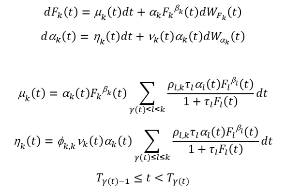
The volatility-of-volatility function νk(t) is a deterministic function of time.
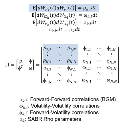
The correlation matrix is 2N-by-2N:
SABR-BGM Correlation Matrix

A special case of null (zero) Forward-Volatility correlations has some advantages:
Sets the Forward-Volatility correlations φk, 1 and the SABR Rho ρk to zero, which means fewer parameters to calibrate
Still fits market data
Gives lower variance and faster convergence in Monte Carlo simulation
To facilitate the calibration of the SABR-BGM model using market data, Rebonato et. al. (2009) introduced the parametric form.
In the parametric form, the SABR volatility αk(t) is decomposed into a product of two components: the deterministic volatility function g(Tk-1 - t) and the stochastic correction term sk(t).
SABR-BGM Model in Rebonato Parametric Form
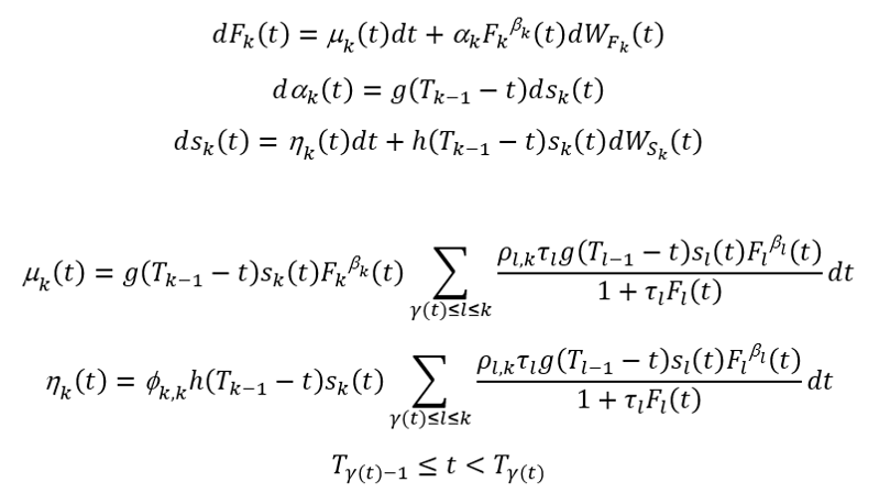
The volatility function g(Tk-1 - t) is a deterministic function of time.
The volatility-of-volatility function h(Tk-1 - t) is a deterministic function of time.
The correlation matrix is 2N-by-2N:
SABR-BGM Model in Rebonato Parametric Form Correlation Matrix
A special case of null (zero) Forward-Volatility correlations has some advantages:
Sets the Forward-Volatility correlations φk, 1 and the SABR Rho ρk to zero, which means fewer parameters to calibrate
Still fits market data
Gives lower variance and faster convergence in Monte Carlo simulation
References
[1] Brigo, D. and F. Mercurio. Interest Rate Models - Theory and Practice. Springer Finance, 2006.
[2] Crispoldi, C., Wigger, G., and P. Larkin. SABR and SABR LIBOR Market Models in Practice. Palgrave MacMillan, 2015.
[3] Hagan, P. and A. Lesniewski. LIBOR market Model with SABR Style Volatility. Working paper JPMorgan Chase, 2008.
[4] Rebonato, R., McKay, K., and R. White. The SABR/LIBOR Market Model: pricing, Calibration, and Hedging for Complex Interest-Rate Derivatives. Wiley, 2009.
Version History
Introduced in R2021b