eigplot
Plot Markov chain eigenvalues
Description
eigplot( creates a plot containing the eigenvalues of the transition matrix of the discrete-time Markov chain mc)mc on the complex plane. The plot highlights the following:
Unit circle
Perron-Frobenius eigenvalue at (1,0)
Circle of second largest eigenvalue magnitude (SLEM)
Spectral gap between the two circles, which determines the mixing time
Examples
Create 10-state Markov chains from two random transition matrices, with one transition matrix being more sparse than the other.
rng(1); % For reproducibility
numstates = 10;
mc1 = mcmix(numstates,'Zeros',20);
mc2 = mcmix(numstates,'Zeros',80); % mc2.P is more sparse than mc1.P
Plot the eigenvalues of the transition matrices on the separate complex planes.
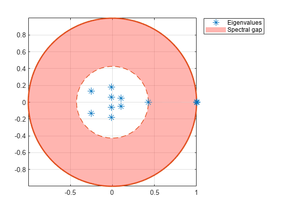
figure;
eigplot(mc1);
figure;
eigplot(mc2);
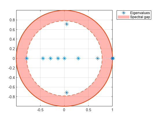
The pink disc in the plots show the spectral gap (the difference between the two largest eigenvalue moduli). The spectral gap determines the mixing time of the Markov chain. Large gaps indicate faster mixing, whereas thin gaps indicate slower mixing. Because the spectral gap of mc1 is thicker than the spectral gap of mc2, mc1 mixes faster than mc2.
Consider this theoretical, right-stochastic transition matrix of a stochastic process.
Create the Markov chain that is characterized by the transition matrix P.
P = [ 0 0 1/2 1/4 1/4 0 0 ;
0 0 1/3 0 2/3 0 0 ;
0 0 0 0 0 1/3 2/3;
0 0 0 0 0 1/2 1/2;
0 0 0 0 0 3/4 1/4;
1/2 1/2 0 0 0 0 0 ;
1/4 3/4 0 0 0 0 0 ];
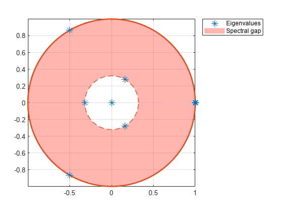
mc = dtmc(P);Plot and return the eigenvalues of the transition matrix on the complex plane.
figure;
eVals = eigplot(mc)
eVals = 7×1 complex

  -0.5000 + 0.8660i
  -0.5000 - 0.8660i
   1.0000 + 0.0000i
  -0.3207 + 0.0000i
   0.1604 + 0.2777i
   0.1604 - 0.2777i
  -0.0000 + 0.0000i
Three eigenvalues have modulus one, which indicates that the period of mc is three.
Compute the mixing time of the Markov chain.
[~,tMix] = asymptotics(mc)
tMix =
0.8793
Input Arguments
Output Arguments
References
[1] Gallager, R.G. Stochastic Processes: Theory for Applications. Cambridge, UK: Cambridge University Press, 2013.
[2] Horn, R., and C. R. Johnson. Matrix Analysis. Cambridge, UK: Cambridge University Press, 1985.
[3] Seneta, E. Non-negative Matrices and Markov Chains. New York, NY: Springer-Verlag, 1981.
Version History
Introduced in R2017b