Compare Markov Chain Mixing Times
This example compares the estimated mixing times of several Markov chains with different structures. Convergence theorems typically require ergodic unichains. Therefore, before comparing mixing time estimates, this example ensures that the Markov chains are ergodic unichains.
Fast-Mixing Chain
Create a 23-state Markov chain from a random transition matrix containing 250 infeasible transitions of 529 total transitions. An infeasible transition is a transition whose probability of occurring is zero. Plot a digraph of the Markov chain and identify classes by using node colors and markers.
rng(1); % For reproducibility
numStates = 23;
Zeros1 = 250;
mc1 = mcmix(numStates,'Zeros',Zeros1);

figure;
graphplot(mc1,'ColorNodes',true);
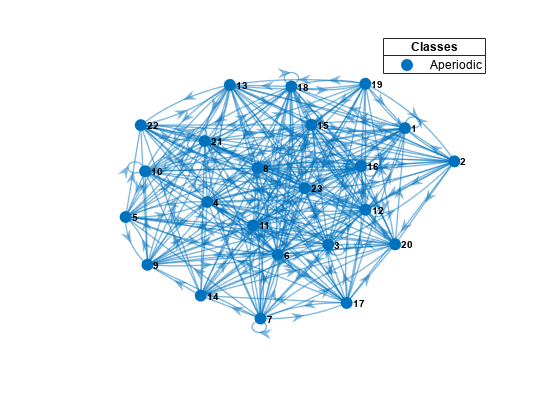
mc1 represents a unichain because it is a single, recurrent, aperiodic class.
Determine whether the Markov chain is ergodic.
tf1 = isergodic(mc1)
tf1 = logical
   1
tf1 = 1 indicates that mc1 represents an ergodic unichain.
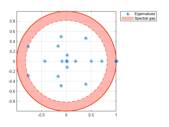
Plot the eigenvalues of the Markov chain on the complex plane.
figure;
eigplot(mc1);
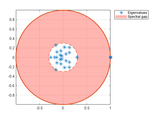
The pink disc in the plot shows the spectral gap (the difference between the two largest eigenvalue moduli). The spectral gap determines the mixing time of the Markov chain. Large gaps indicate faster mixing, whereas thin gaps indicate slower mixing. In this case, the gap is large, indicating a fast-mixing chain.
Estimate the mixing time of the chain.
[~,tMix1] = asymptotics(mc1)
tMix1 =
0.8357
On average, it takes 0.8357 steps for the total variation distance to decay by a factor of .
The expected first hitting time for a target state is another way to view the mixing rate of a Markov chain. The hitting time computation does not require an ergodic Markov chain.
Plot a digraph of the Markov chain with node colors representing the expected first hitting times for regime 1.
hittime(mc1,1,'Graph',true);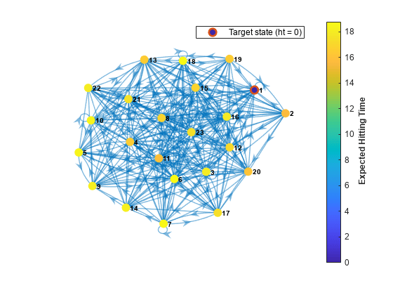
The expected first hitting time for regime 1 beginning from regime 2 is approximately 16 time steps.
Slow-Mixing Chain
Create another 23-state Markov chain from a random transition matrix containing 475 infeasible transitions. With fewer feasible transitions, this chain should take longer to mix. Plot a digraph of the Markov chain and identify classes by using node colors and markers.
Zeros2 = 475;
mc2 = mcmix(numStates,'Zeros',Zeros2);

figure;
graphplot(mc2,'ColorNodes',true);
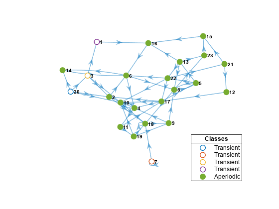
mc2 represents a unichain because it has a single, recurrent, aperiodic class and several transient classes.
Determine whether the Markov chain is ergodic.
tf2 = isergodic(mc2)
tf2 = logical
   0
tf2 = 0 indicates that mc2 is not ergodic.
Extract the recurrent subchain from mc2. Determine whether the subchain is ergodic.
[bins,~,ClassRecurrence] = classify(mc2);
recurrentClass = find(ClassRecurrence,1);
recurrentState = find((bins == recurrentClass),1);
sc2 = subchain(mc2,recurrentState);
tf2 = isergodic(sc2)
tf2 = logical
   1
sc2 represents an ergodic unichain.
Plot the eigenvalues of the subchain on the complex plane.
figure;
eigplot(sc2);
The spectral gap in the subchain is much thinner than the gap in mc1, which indicates that the subchain mixes more slowly.
Estimate the mixing time of the subchain.
[~,tMix2] = asymptotics(sc2)
tMix2 =
5.0201
On average, it takes 5.0201 steps for the total variation distance to decay by a factor of .
Plot a digraph of the Markov chain with node colors representing the expected first hitting times for the first regime in the recurrent subclass.
sc2.StateNames(1)
ans =
"2"
hittime(sc2,1,'Graph',true);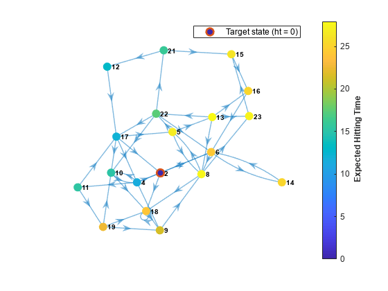
The expected first hitting time for regime 2 beginning from regime 8 is about 30 time steps.
Dumbbell Chain Mixing Time
Create a "dumbbell" Markov chain containing 10 states in each "weight" and three states in the "bar."
Specify random transition probabilities between states within each weight.
If the Markov chain reaches the state in a weight that is closest to the bar, then specify a high probability of transitioning to the bar.
Specify uniform transitions between states in the bar.
w = 10;                             % Dumbbell weights
DBar = [0 1 0; 1 0 1; 0 1 0];       % Dumbbell bar
DB = blkdiag(rand(w),DBar,rand(w)); % Transition matrix

% Connect dumbbell weights and bar
DB(w,w+1) = 1;
DB(w+1,w) = 1;
DB(w+3,w+4) = 1;
DB(w+4,w+3) = 1;

mc3 = dtmc(DB);
Plot a directed graph of the dumbbell chain and identify classes by using node colors and markers. Suppress node labels.
figure;
h = graphplot(mc3,'ColorNodes',true);
h.NodeLabel = {};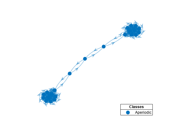
mc3 represents a unichain because it has a single, recurrent, aperiodic class.
Determine whether the Markov chain is ergodic.
tf3 = isergodic(mc3)
tf3 = logical
   1
tf3 = 1 indicates that mc3 is ergodic.
Plot the eigenvalues of the dumbbell on the complex plane.
figure;
eigplot(mc3);
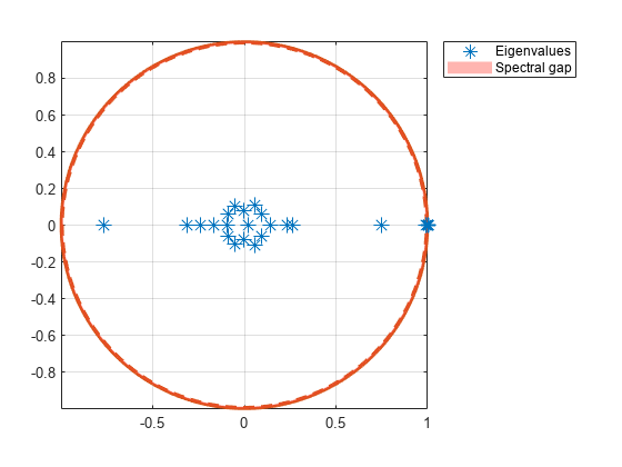
The spectral gap in the subchain is very thin, which indicates that the dumbbell chain mixes very slowly.
Estimate the mixing time of the dumbbell chain.
[~,tMix3] = asymptotics(mc3)
tMix3 =
90.4334
On average, it takes 90.4334 steps for the total variation distance to decay by a factor of .
Plot a digraph of the Markov chain with node colors representing the expected first hitting times for regime 1.
hittime(mc3,1,'Graph',true);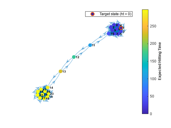
The expected first hitting time for regime 1 beginning from regime 15 is about 300 time steps.