filter
Filter disturbances using univariate ARIMA or ARIMAX model
Description
Y = filter(Mdl,Z)Y resulting
from filtering the numeric array of one or more underlying disturbance series
Z through the fully specified, univariate ARIMA model
Mdl. Z is associated with the model innovations
process that drives the specified ARIMA model.
Tbl2 = filter(Mdl,Tbl1)Tbl2 containing the results from
filtering the paths of disturbances in the input table or timetable
Tbl1 through Mdl. The disturbance variable in
Tbl1 is associated with the model innovations process through
Mdl. (since R2023b)
filter selects the variable
Mdl.SeriesName, or the sole variable in Tbl1, as
the disturbance variable to filter through the model. To select a different variable in
Tbl1 to filter through the model, use the
DisturbanceVariable name-value argument.
[___] = filter(___,
specifies options using one or more name-value arguments in
addition to any of the input argument combinations in previous syntaxes.
Name,Value)filter returns the output argument combination for the
corresponding input arguments. For example, filter(Mdl,Z,Z0=PS,X=Pred) filters the
numeric vector of disturbances Z through the ARIMAX
Mdl, and specifies the numeric vector of presample disturbance data
PS to initialize the model and the exogenous predictor data
X for the regression component.
Examples
Compute the impulse response function (IRF) of an ARMA model by filtering a vector of zeros, representing disturbances, through the model.
Specify a mean zero ARMA(2,0,1) model.
Mdl = arima(Constant=0,AR={0.5 -0.8},MA=-0.5, ...
    Variance=0.1);
Simulate the first 20 responses of the IRF. Generate a disturbance series with a one-time, unit impulse, and then filter it.
z = [1; zeros(19,1)];
y = filter(Mdl,z);
y is a 20-by-1 response path resulting from filtering the disturbance path z through the model. y represents the IRF. The filter function requires one presample observation to initialize the model. By default, filter uses the unconditional mean of the process, which is 0.
y = y/y(1);
Normalize the IRF such that the first element is 1.
Plot the impulse response function.
figure
stem((0:numel(y)-1)',y,"filled");
title("Impulse Response")
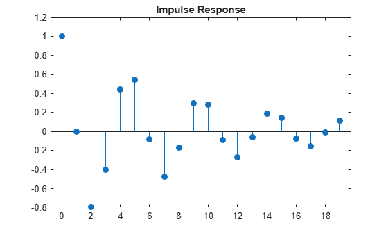
The impulse response assesses the dynamic behavior of a system to a one-time, unit impulse.
Alternatively, you can use the impulse function to plot the IRF for an ARIMA process.
Filter a matrix of disturbance paths. Return the paths of responses and innovations, which drive the data-generating processes.
Create a mean zero ARIMA(2,0,1) model.
Mdl = arima(Constant=0,AR={0.5,-0.8},MA=-0.5, ...
    Variance=0.1);
Generate 20 random, length 100 paths from the model.
rng(1,"twister"); % For reproducibility
[ySim,eSim,vSim] = simulate(Mdl,100,NumPaths=20);
ySim, eSim, and vSim are 100-by-20 matrices of 20 simulated response, innovation, and conditional variance paths of length 100, respectively. Because Mdl does not have a conditional variance model, vSim is a matrix completely composed of the value of Mdl.Variance.
Obtain disturbance paths by standardizing the simulated innovations.
zSim = eSim./sqrt(vSim);
Filter the disturbance paths through the model.
[yFil,eFil] = filter(Mdl,zSim);
yFil and eFil are 100-by-20 matrices. The columns are independent paths generated from filtering corresponding disturbance paths in zSim through the model Mdl.
Confirm that the outputs of simulate and filter are identical.
sameE = norm(eSim - eFil) < eps
sameE = logical
   1
sameY = norm(ySim - yFil) < eps
sameY = logical
   1
The logical values 1 confirm the outputs are effectively identical.
Since R2023b
Fit an ARIMA(1,1,1) model to the weekly average NYSE closing prices. Supply a timetable of data and specify the series for the fit. Then, filter randomly generated Gaussian noise paths through the estimated model to simulate responses and innovations.
Load Data
Load the US equity index data set Data_EquityIdx.
load Data_EquityIdx
T = height(DataTimeTable)
T = 3028
The timetable DataTimeTable includes the time series variable NYSE, which contains daily NYSE composite closing prices from January 1990 through December 2001.
Plot the daily NYSE price series.
figure
plot(DataTimeTable.Time,DataTimeTable.NYSE)
title("NYSE Daily Closing Prices: 1990 - 2001")
Prepare Timetable for Estimation
When you plan to supply a timetable, you must ensure it has all the following characteristics:
The selected response variable is numeric and does not contain any missing values.
The timestamps in the
Timevariable are regular, and they are ascending or descending.
Remove all missing values from the timetable, relative to the NYSE price series.
DTT = rmmissing(DataTimeTable,DataVariables="NYSE");
T_DTT = height(DTT)
T_DTT = 3028
Because all sample times have observed NYSE prices, rmmissing does not remove any observations.
Determine whether the sampling timestamps have a regular frequency and are sorted.
areTimestampsRegular = isregular(DTT,"days")areTimestampsRegular = logical
0
areTimestampsSorted = issorted(DTT.Time)
areTimestampsSorted = logical
   1
areTimestampsRegular = 0 indicates that the timestamps of DTT are irregular. areTimestampsSorted = 1 indicates that the timestamps are sorted. Business day rules make daily macroeconomic measurements irregular.
Remedy the time irregularity by computing the weekly average closing price series of all timetable variables.
DTTW = convert2weekly(DTT,Aggregation="mean");
areTimestampsRegular = isregular(DTTW,"weeks")
areTimestampsRegular = logical
   1
T_DTTW = height(DTTW)
T_DTTW =
627
DTTW is regular.
figure
plot(DTTW.Time,DTTW.NYSE)
title("NYSE Daily Closing Prices: 1990 - 2001")
Create Model Template for Estimation
Suppose that an ARIMA(1,1,1) model is appropriate to model NYSE composite series during the sample period.
Create an ARIMA(1,1,1) model template for estimation. Set the response series name to NYSE.
Mdl = arima(1,1,1);
Mdl.SeriesName = "NYSE";
Mdl is a partially specified arima model object.
Fit Model to Data
Fit an ARIMA(1,1,1) model to weekly average NYSE closing prices. Specify the entire series.
EstMdl = estimate(Mdl,DTTW);
    ARIMA(1,1,1) Model (Gaussian Distribution):

                 Value      StandardError    TStatistic      PValue
                ________    _____________    __________    ___________

    Constant     0.86385       0.46496         1.8579         0.063181
    AR{1}       -0.37582       0.22719        -1.6542          0.09809
    MA{1}        0.47221       0.21741          2.172         0.029859
    Variance       55.89         1.832         30.507      2.1201e-204
EstMdl is a fully specified, estimated arima model object. By default, estimate backcasts for the required Mdl.P = 2 presample responses.
Filter Random Gaussian Disturbance Paths
Generate 2 random, independent series of length T_DTTW from the standard Gaussian distribution. Store the matrix of series as one variable in DTTW.
rng(1,"twister") % For reproducibility
DTTW.Z = randn(T_DTTW,2);
DTTW contains a new variable called Z containing a T_DTTW-by-2 matrix of two disturbance paths.
Filter the paths of disturbances through the estimated ARIMA model. Specify the table variable name containing the disturbance paths.
Tbl2 = filter(EstMdl,DTTW,DisturbanceVariable="Z");
tail(Tbl2)
Time NYSE NASDAQ Z NYSE_Response NYSE_Innovation NYSE_Variance
___________ ______ ______ _____________________ ________________ ___________________ ______________
16-Nov-2001 577.11 1886.9 -1.8948 0.41292 358.78 433.57 -14.166 3.087 55.89 55.89
23-Nov-2001 583 1898.3 1.3583 0.27051 367.95 436.63 10.155 2.0223 55.89 55.89
30-Nov-2001 581.41 1925.8 -0.9118 1.1119 363.35 445.61 -6.8165 8.3125 55.89 55.89
07-Dec-2001 584.96 1998.1 -0.14964 -2.418 361.61 428.95 -1.1187 -18.077 55.89 55.89
14-Dec-2001 574.03 1981 -0.40114 0.98498 359.6 434.9 -2.9989 7.3636 55.89 55.89
21-Dec-2001 582.1 1967.9 -0.57758 0.0039243 355.48 437.03 -4.318 0.029338 55.89 55.89
28-Dec-2001 590.28 1967.2 2.0039 -0.92415 370.83 430.2 14.981 -6.9089 55.89 55.89
04-Jan-2002 589.8 1950.4 -0.50964 -0.43856 369.19 427.09 -3.8101 -3.2787 55.89 55.89
size(Tbl2)
ans = 1×2

   627     6
Tbl2 is a 627-by-6 timetable containing all variables in DTTW, and the two filtered response paths NYSE_Response, innovation paths NYSE_Innovation, and constant variance paths NYSE_Variance (Mdl.Variance = 55.89).
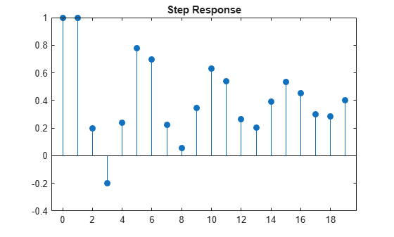
Assess the dynamic behavior of a system to a persistent change in a variable by plotting a step response. Supply presample responses to initialize the model.
Specify a mean zero ARIMA(2,0,1) process.
Mdl = arima(Constant=0,AR={0.5 -0.8},MA=-0.5, ...
    Variance=0.1);
Simulate the first 20 responses to a sequence of unit disturbances. Generate a disturbance series of ones, and then filter it. Set all presample observations equal to zero.
Z = ones(20,1);
Y = filter(Mdl,Z,Y0=zeros(Mdl.P,1));
Y = Y/Y(1);
The last step normalizes the step response function to ensure that the first element is 1.
Plot the step response function.
figure
stem((0:numel(Y)-1)',Y,"filled");
title("Step Response")
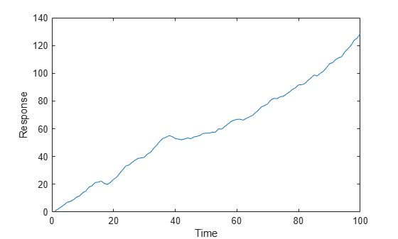
Create models for the response and predictor series. Set an ARIMAX(2,1,3) model to the response MdlY, and an AR(1) model to the MdlX.
MdlY = arima(AR={0.1 0.2},D=1,MA={-0.1 0.1 0.05}, ...
    Constant=1,Variance=0.5,Beta=2);
MdlX = arima(AR=0.5,Constant=0,Variance=0.1);
Simulate a length 100 predictor series x and a series of iid normal disturbances z having mean zero and variance 1.
rng(1,"twister")
z = randn(100,1);
x = simulate(MdlX,100);
Filter the disturbances z using MdlY to produce the response series y. Plot y.
y = filter(MdlY,z,X=x);
figure
plot(y);
xlabel("Time")
ylabel("Response")
Create the composite AR(1)/GARCH(1,1) model
Create the composite model.
CVMdl = garch(Constant=0.2,GARCH=0.1,ARCH=0.05);
Mdl = arima(Constant=1,AR=0.5,Variance=CVMdl)
Mdl =
  arima with properties:

     Description: "ARIMA(1,0,0) Model (Gaussian Distribution)"
      SeriesName: "Y"
    Distribution: Name = "Gaussian"
               P: 1
               D: 0
               Q: 0
        Constant: 1
              AR: {0.5} at lag [1]
             SAR: {}
              MA: {}
             SMA: {}
     Seasonality: 0
            Beta: [1×0]
        Variance: [GARCH(1,1) Model]
Mdl is an arima object. The property Mdl.Variance contains a garch object that represents the conditional variance model.
Generate a random series of 100 standard Gaussian of disturbances.
rng(1,"twister") % For reproducibility
z = randn(100,1);
Filter the disturbances through the model. Return and plot the simulated conditional variances.
[y,e,v] = filter(Mdl,z);
plot(z)

Input Arguments
Name-Value Arguments
Output Arguments
Alternative Functionality
filter generalizes simulate; both functions filter a series of disturbances to produce output
responses, innovations, and conditional variances. However, simulate
autogenerates a series of mean zero, unit variance, independent and identically distributed
(iid) disturbances according to the distribution in Mdl. In contrast,
filter enables you to directly specify custom disturbances.
References
[1] Box, George E. P., Gwilym M. Jenkins, and Gregory C. Reinsel. Time Series Analysis: Forecasting and Control. 3rd ed. Englewood Cliffs, NJ: Prentice Hall, 1994.
[2] Enders, Walter. Applied Econometric Time Series. Hoboken, NJ: John Wiley & Sons, Inc., 1995.
[3] Hamilton, James D. Time Series Analysis. Princeton, NJ: Princeton University Press, 1994.