Main Content

dsp.ISTFT

Inverse short-time FFT

Description

The dsp.ISTFT object computes the inverse short-time Fourier transform (ISTFT) of the frequency-domain input signal and returns the time-domain output. The object accepts frames of Fourier-transformed data, converts these frames into the time domain using the IFFT operation, and performs overlap-add to reconstruct the data. The output of the object is the reconstructed signal normalized by a factor that depends on the hop length and sum(window). For more details, see Algorithms.

Creation

Description

istf = dsp.ISTFT returns an object, istf, that implements inverse short-time FFT. The object processes the data independently across each input channel over time.

istf = dsp.ISTFT(window) returns an inverse short-time FFT object with the Window property set to window.

istf = dsp.ISTFT(window,overlap) returns an inverse short-time FFT object with the Window property set to window and the OverlapLength property set to overlap.

istf = dsp.ISTFT(window,overlap,isconjsym) returns an inverse short-time FFT object with the Window property set to window, OverlapLength property set to overlap, and the ConjugateSymmetricInput property set to isconjsym.

istf = dsp.ISTFT(window,overlap,isconjsym,woa) returns an inverse short-time FFT object with the Window property set to window, with the OverlapLength property set to overlap, the ConjugateSymmetricInput property set to isconjsym, and the WeightedOverlapAdd property set to woa.

istf = dsp.ISTFT(Name,Value) returns an inverse short-time FFT object with each specified property name set to the specified value. You can specify additional name-value pair arguments in any order.

Properties

expand all

Synthesis window, specified as a vector of real elements.

Tunable: Yes

Data Types: single | double

Number of samples by which consecutive windows overlap, specified as a positive integer. The windows overlap to reduce the artifacts at the data boundaries.

Hop length is the difference between the window length and the overlap length.

Data Types: single | double | int8 | int16 | int32 | int64 | uint8 | uint16 | uint32 | uint64

Set this property to true if the input is conjugate symmetric, which yields real-valued outputs. The FFT of a real-valued signal is conjugate symmetric, and setting this property to true optimizes the IFFT computation method. Setting this property to false for conjugate symmetric inputs results in complex output values with small imaginary parts. Setting this property to true for non-conjugate symmetric inputs results in invalid outputs.

Data Types: logical

Set this property to true to apply weighted overlap-add. In weighted overlap-add, the IFFT output is multiplied by the window before overlap-add. Set this property to false to skip multiplication by the window.

Data Types: logical

Specify the frequency range as 'onesided' or 'twosided'. If you set the FrequencyRange property to:

  • 'twosided' –– The inverse short-time FFT is computed for a two-sided short-time FFT. The FFT length used is equal to the input frame length.

  • 'onesided' –– The one-sided inverse short-time FFT is computed for a one-sided short-time FFT. If the input frame length is odd, the FFT length used is (frame length − 1) × 2. If the input frame length is even, the FFT length used is (frame length × 2) − 1.

Usage

Description

example

y = istft(x) applies inverse short-time FFT on the input x, and returns the time-domain output y.

Input Arguments

expand all

Frequency-domain input signal, specified as a vector or a matrix. If the input is a matrix, the object treats each column as an independent channel. The FFT length is equal to the number of rows of x. The FFT length, hence the number of input rows must be greater than or equal to the window length.

Data Types: single | double
Complex Number Support: Yes

Output Arguments

expand all

Inverse short-time FFT output, returned as a vector or a matrix. The output frame length (number of rows in y) is equal to WLOL, where WL is the window length and OL is the overlap length.

The output is complex with small imaginary parts when the input x is conjugate symmetric and the ConjugateSymmetricInput property is set to false. The data type of the output matches the data type of the input signal.

Data Types: single | double
Complex Number Support: Yes

Object Functions

stepRun System object algorithm
releaseRelease resources and allow changes to System object property values and input characteristics
resetReset internal states of System object
cloneCreate duplicate System object
isLockedDetermine if System object is in use

Examples

collapse all

Short-time spectral attenuation is achieved by applying a time-varying attenuation to the short-time spectrum of a noisy signal. The gain of the attenuation is determined by the estimate of the noise power in each subband of the spectrum. This gain, when applied to the noisy spectrum, attenuates the subbands with higher noise power and lifters the subbands with lesser noise power.

Here are the steps involved in performing the short-time spectral attenuation:

  1. Analyze the noisy input signal by computing the short-time Fourier transform (STFT).

  2. Multiply each subband of the transformed signal with a real positive gain less than 1.

  3. Synthesize the denoised subbands by taking the inverse short-time Fourier transform (ISTFT). The resconstructed signal is the denoised input signal.

Use the dsp.STFT and dsp.ISTFT objects to compute the short-time and the inverse short-time Fourier transforms, respectively.

Noisy Input Signal

The input is an audio signal sampled at the 22,050 Hz. The dsp.AudioFileReader object reads this signal in frames of 512 samples. The audio signal is corrupted by white Gaussian noise that has a standard deviation of 0.05. Use the audioDeviceWriter object to play the noisy audio signal to your computer's audio device.

FrameLength = 512;
afr = dsp.AudioFileReader('speech_dft.wav',...
    'SamplesPerFrame',FrameLength);
adw = audioDeviceWriter('SampleRate',afr.SampleRate);

noiseStd = 0.05;
while ~isDone(afr)
    cleanAudio = afr();
    noisyAudio = cleanAudio + noiseStd * randn(FrameLength,1);
    adw(noisyAudio);
end
reset(afr)

Initialize Short-Time and Inverse Short-Time Fourier Transform Objects

Initialize the dsp.STFT and dsp.ISTFT objects. Set the window length equal to the input frame length and the hop length to 16. The overlap length is the difference between the window length and the hop length, OL = WLHL. Set the FFT length to 1024.

WindowLength = FrameLength;
HopLength = 16;
numHopsPerFrame = FrameLength / 16;
FFTLength = 1024;

The window used to compute the STFT and ISTFT is a periodic hamming window with length 512. The ConjugateSymmetricInput flag of the istf object is set to true, indicating that the output of the istf object is a conjugate-symmetric signal.

win = hamming(WindowLength,'periodic');
stf = dsp.STFT(win,WindowLength-HopLength,FFTLength);
istf = dsp.ISTFT(win,WindowLength-HopLength,1,0);

Gain Estimator

The next step is to define the gain estimator parameters. This gain is applied to the noisy spectrum to attenuate the subbands with higher noise power and lifter the subbands with lesser noise power.

dec = 16;
alpha = 15;
stftNorm = (sum(win.*win) / dec).^2;

Spectral Attenuation

Feed the audio signal to stf one hop-length at a time. Apply the estimated gain to the transformed signal. Reconstruct the denoised version of the original speech signal by performing an inverse Fourier transform on the individual frequency bands. Play the denoised audio signal to the computer's audio device.

while ~isDone(afr)
    cleanAudio =  afr();
    noisyAudio = cleanAudio + noiseStd * randn(FrameLength,1);
    y = zeros(FrameLength,1); % y holds the denoised audio frame
    
    % Feed audio to stft one hop-length at a time
    for index = 1:numHopsPerFrame        
        X = stf(noisyAudio((index-1)*HopLength+1:index*HopLength));        
        % Gain estimator
        Z = abs(X).^2 / (noiseStd^2 * alpha) / stftNorm;
        Z(Z<=1) = 1;
        Z = 1 - 1./Z;
        Z = sign(Z) .* sqrt(abs(Z));
        X = X .* Z;        
        % Convert back to time-domain
        y((index-1)*HopLength+1:index*HopLength) = istf(X);        
    end    
    % Listen to denoised audio:
    adw(y);
end

Perfect reconstruction is when the output of dsp.ISTFT matches the input to dsp.STFT. Perfect reconstruction is obtained if the analysis window, g(n), obeys the constant overlap-add (COLA) property at hop-size R.

m=-g(n-mR)=1,nΖ     (gCOLA(R))

A signal is perfectly reconstructed if the output of the dsp.ISTFT object matches the input to the dsp.STFT object.

iscola Function

The iscola function checks that the specified window and overlap satisfy the COLA constraint to ensure that the inverse short-time Fourier transform (ISTFT) results in perfect reconstruction for non-modified spectra. The function returns a logical true if the combination of input parameters is COLA-compliant and a logical false if not. The method argument of the function is set to 'ola' or 'wola' depending on whether the inversion method uses weighted overlap-add (WOLA).

Check if hann() window of length 120 samples and an overlap length of 60 samples is COLA compliant.

winLen = 120;
overlapLen = 60;
win = hann(winLen,'periodic');
tf = iscola(win,overlapLen,'ola')
tf = logical
   1

Initialization

Initialize the dsp.STFT and dsp.ISTFT System objects with this hann window that is COLA compliant. Set the FFT length to equal the window length.

frameLen = winLen-overlapLen;
stf = dsp.STFT('Window',win,'OverlapLength',overlapLen,'FFTLength',winLen);
istf = dsp.ISTFT('Window',win,'OverlapLength',overlapLen,'WeightedOverlapAdd',0);

Reconstruct Data

Compute the STFT of a random signal. Set the length of the input signal to equal the hop length (window length – overlap length). Since the window is COLA compliant, the ISTFT of this non-modified spectra perfectly reconstructs the original time-domain signal.

To confirm, compare the input, x to the reconstructed output, y. Due to the latency introduced by the objects, the reconstructed output is shifted in time compared to the input. Therefore, to compare, take the norm of the difference between the reconstructed output, y and the previous input, xprev. The norm is very small, indicating that the output signal is a perfectly reconstructed version of the input signal.

n = zeros(1,100);
xprev = 0;
for i = 1:100
    x = randn(frameLen,1);
    X = stf(x);
    y = istf(X);
    n(1,i) = norm(y-xprev);
    xprev = x;
end       
max(abs(n))
ans = 1.6972e-13

ISTFT with Weighted Overlap-Add (WOLA)

In WOLA, a second window called the synthesis window, f(n), is applied after the IFFT operation and before overlap-add. The synthesis and analysis windows are typically identical and are usually obtained by taking the square root of windows satisfying COLA (thereby ensuring perfect reconstruction).

iscola Function

Check if sqrt(hann()) window of length 120 samples and an overlap length of 60 samples is WOLA compliant. Set the method argument of the iscola function to 'wola'. The output of the iscola function is 1 indicating that this window is WOLA compliant.

winWOLA = sqrt(hann(winLen,'periodic'));
tfWOLA = iscola(winWOLA,overlapLen,'wola')
tfWOLA = logical
   1

Reconstruct Data with WOLA

Release the dsp.STFT and dsp.ISTFT System objects and set the window to sqrt(hann(winLen,'periodic')) window. To use weighted overlap-add on the ISTFT side, set the 'WeightedOverlapAdd' to true.

release(stf);
release(istf);
stf.Window = winWOLA;
istf.Window = winWOLA;
istf.WeightedOverlapAdd = true;

n = zeros(1,100);
xprev = 0;
for i = 1:100
    x = randn(frameLen,1);
    X = stf(x);
    y = istf(X);
    n(1,i) = norm(y-xprev);
    xprev = x;
end       
max(abs(n))
ans = 4.6664e-15

The norm of the difference between the input signal and the reconstructed signal is very small indicating that the signal has been reconstructed perfectly.

More About

expand all

Algorithms

Here is a sketch of how the algorithm is implemented without weighted overlap-add (WOLA):

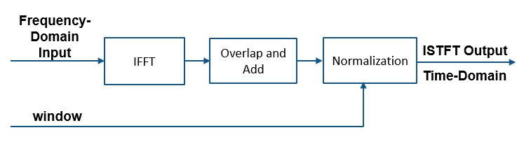
The frequency-domain input is inverted using IFFT, and then overlap-add is performed. Note that each run of the algorithm generates R new output time-domain samples, where R is the hop length. The hop length is defined as WLOL, where WL is the window length and OL is the overlap length. The normalization stage multiplies the output by R/sum(win), where win is the window vector specified in the Window property.

Here is a sketch of how the algorithm is implemented with Weighted Overlap-Add (WOLA):

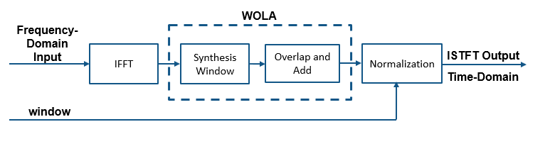
In WOLA, a second window (usually called the synthesis window) is applied after the IFFT operation and before overlap-add. WOLA is used to suppress discontinuities at frame boundaries caused by nonlinear processing of the STFT. For more details, see More About.

Here is an illustration of how the input frequency subbands look when inverted with IFFT and overlap-added together to reconstruct a time-domain signal.

The analysis window (on the STFT side) and the synthesis window (on the ISTFT side) are typically identical. To ensure perfect reconstruction, the windows are usually obtained by taking the square root of windows satisfying the constant overlap-add (COLA) property. For details on the COLA property and how perfect reconstruction is defined, see the More About in dsp.STFT page.

References

[1] Allen, J.B., and L. R. Rabiner. "A Unified Approach to Short-Time Fourier Analysis and Synthesis,'' Proceedings of the IEEE, Vol. 65, pp. 1558–1564, Nov. 1977.

Extended Capabilities

Version History

Introduced in R2019a

See Also

Objects

Blocks