Create Driving Scenario Programmatically
This example shows how to generate ground truth for synthetic sensor data and tracking algorithms. It also shows how to update actor poses in open-loop and closed-loop simulations. Finally, it shows how to use the driving scenario to perform coordinate conversion and incorporate them into the bird's-eye plot.
In this example, you programmatically create the driving scenario from the MATLAB® command line. Alternatively, you can create scenarios interactively by using the Driving Scenario Designer app. For an example, see Create Driving Scenario Interactively and Generate Synthetic Sensor Data.
Introduction
One of the goals of a driving scenario is to generate "ground truth" test cases for use with sensor detection and tracking algorithms used on a specific vehicle.
This ground truth is typically defined in a global coordinate system; but, because sensors are typically mounted on a moving vehicle, this data needs to be converted to a reference frame that moves along with the vehicle. The driving scenario facilitates this conversion automatically, allowing you to specify roads and trajectories of objects in global coordinates and provides tools to convert and visualize this information in the reference frame of any actor in the scenario.
Convert Pose Information to an Actor's Reference Frame
A drivingScenario consists of a model of roads and movable objects, called actors. You can use actors to model pedestrians, parking meters, fire hydrants, and other objects within the scenario. Actors consist of cuboids with a length, width, height, and a radar cross-section (RCS). An actor is positioned and oriented about a single point in the center of its bottom face.
A special kind of actor that moves on wheels is a vehicle, which is positioned and oriented on the ground directly beneath the center of the rear axle, which is a more natural center of rotation.
All actors (including vehicles) may be placed anywhere within the scenario by specifying their respective Position, Roll, Pitch, Yaw, Velocity, and AngularVelocity properties.
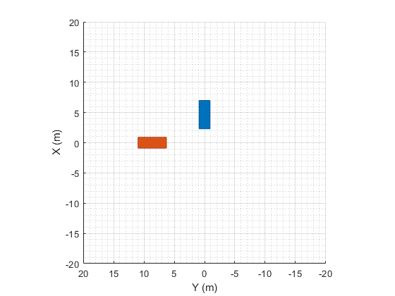
Here is an example of a scenario consisting of two vehicles 10 meters apart and driving towards the origin at a speed of 3 and 4 meters per second, respectively:
scenario = drivingScenario;
v1 = vehicle(scenario,'ClassID',1','Position',[6 0 0],'Velocity',[-3 0 0],'Yaw',180)
v1 =

  Vehicle with properties:

         FrontOverhang: 0.9000
          RearOverhang: 1
             Wheelbase: 2.8000
             EntryTime: 0
              ExitTime: Inf
               ActorID: 1
               ClassID: 1
                  Name: ""
             AssetType: "Unspecified"
             AssetPath: ""
             PlotColor: [0.0660 0.4430 0.7450]
              Position: [6 0 0]
              Velocity: [-3 0 0]
                   Yaw: 180
                 Pitch: 0
                  Roll: 0
       AngularVelocity: [0 0 0]
                Length: 4.7000
                 Width: 1.8000
                Height: 1.4000
                  Mesh: [1×1 extendedObjectMesh]
            RCSPattern: [2×2 double]
      RCSAzimuthAngles: [-180 180]
    RCSElevationAngles: [-90 90]
v2 = vehicle(scenario,'ClassID',1,'Position',[0 10 0],'Velocity',[0 -4 0],'Yaw',-90)
v2 =

  Vehicle with properties:

         FrontOverhang: 0.9000
          RearOverhang: 1
             Wheelbase: 2.8000
             EntryTime: 0
              ExitTime: Inf
               ActorID: 2
               ClassID: 1
                  Name: ""
             AssetType: "Unspecified"
             AssetPath: ""
             PlotColor: [0.8660 0.3290 0]
              Position: [0 10 0]
              Velocity: [0 -4 0]
                   Yaw: -90
                 Pitch: 0
                  Roll: 0
       AngularVelocity: [0 0 0]
                Length: 4.7000
                 Width: 1.8000
                Height: 1.4000
                  Mesh: [1×1 extendedObjectMesh]
            RCSPattern: [2×2 double]
      RCSAzimuthAngles: [-180 180]
    RCSElevationAngles: [-90 90]
To visualize a scenario, call the plot function on it:
plot(scenario);
set(gcf,'Name','Scenario Plot')
xlim([-20 20]);
ylim([-20 20]);
Once all the actors in a scenario have been created, you can inspect the pose information of all the actors in the coordinates of the scenario by inspecting the Position, Roll, Pitch, Yaw, Velocity, and AngularVelocity properties of each actor, or you may obtain all of them in a convenient structure by calling the actorPoses function on the scenario:
ap = actorPoses(scenario)
ap =

  2×1 struct array with fields:

    ActorID
    Position
    Velocity
    Roll
    Pitch
    Yaw
    AngularVelocity
To obtain the pose information of all other objects (or targets) seen by a specific actor in its own reference frame, you can call the targetPoses function on the actor itself:
v2TargetPoses = targetPoses(v2)
v2TargetPoses =

  struct with fields:

            ActorID: 1
            ClassID: 1
           Position: [10 6.0000 0]
           Velocity: [-4 -3.0000 0]
               Roll: 0
              Pitch: 0
                Yaw: -90.0000
    AngularVelocity: [0 0 0]
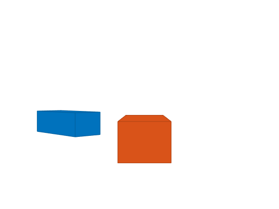
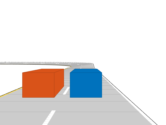
We can qualitatively confirm the relative vehicle placement by adding a chase plot for a vehicle. By default, a chase plot displays a projective-perspective view from a fixed distance behind the vehicle.
Here we show the perspective seen just behind the second vehicle (red). The target poses seen by the second vehicle show that the location of the other vehicle (in blue) is 6 m forward and 10 m to the left of the second vehicle. We can see this qualitatively in the chase plot:
chasePlot(v2)
set(gcf,'Name','Chase Plot')

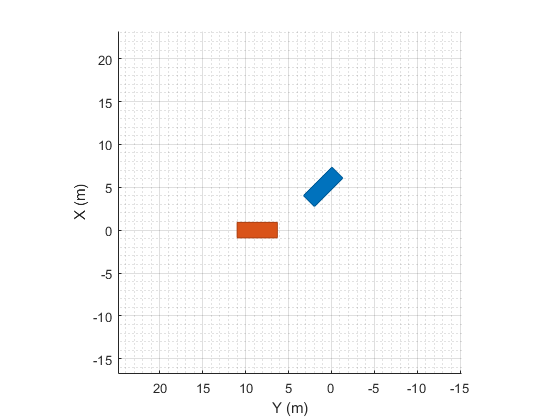
Normally all plots associated with a driving scenario are updated in the course of simulation when calling the advance function. If you update a position property of another actor manually, you can call updatePlots to see the results immediately:
v1.Yaw = 135;
updatePlots(scenario);
Convert Road Boundaries to an Actor's Reference Frame
The driving scenario can also be used to retrieve the boundaries of roads defined in the scenario.
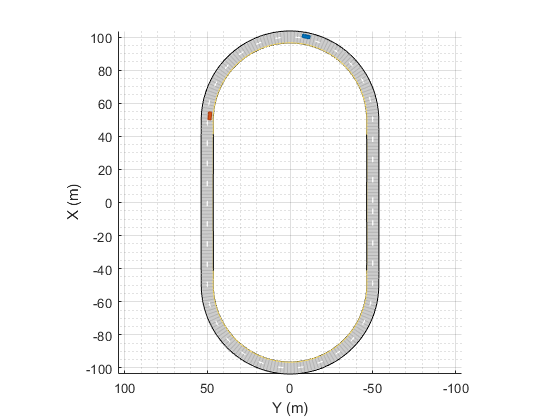
Here we make use of the simple oval track described in Define Road Layouts Programmatically, which covers an area roughly 200 meters long and 100 meters wide and whose curves have a bank angle of nine degrees:
scenario = drivingScenario;
roadCenters = ...
    [  0  40  49  50 100  50  49 40 -40 -49 -50 -100  -50  -49  -40    0
     -50 -50 -50 -50   0  50  50 50  50  50  50    0  -50  -50  -50  -50
       0   0 .45 .45 .45 .45 .45  0   0 .45 .45  .45  .45  .45    0    0]';
bankAngles = ...
    [  0   0   9   9   9   9   9  0   0   9   9    9    9    9    0    0];

road(scenario, roadCenters, bankAngles, 'lanes', lanespec(2));
plot(scenario);
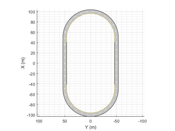
To obtain the lines that define the borders of the road, use the roadBoundaries function on the driving scenario. It returns a cell array that contains the road borders (shown in the scenario plot above as the solid black lines).
rb = roadBoundaries(scenario)
rb =

  1×2 cell array

    {258×3 double}    {258×3 double}
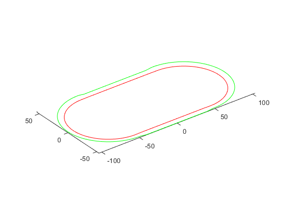
In the example above, there are two road boundaries (an outer and an inner boundary). You can plot them yourself as follows:
figure

outerBoundary = rb{1};
innerBoundary = rb{2};

plot3(innerBoundary(:,1),innerBoundary(:,2),innerBoundary(:,3),'r', ...
      outerBoundary(:,1),outerBoundary(:,2),outerBoundary(:,3),'g')
axis equal
You can use the roadBoundaries function on an actor to obtain the road boundaries in the coordinates of the actor. To do that, simply pass the actor as the first argument, instead of the scenario.
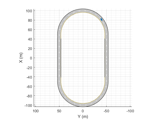
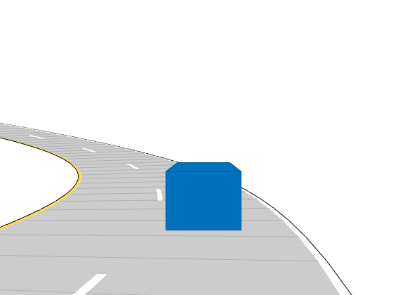
To see this, add an "ego vehicle" and place it on the track:
egoCar = vehicle(scenario,'ClassID',1,'Position',[80 -40 0.45],'Yaw',30);
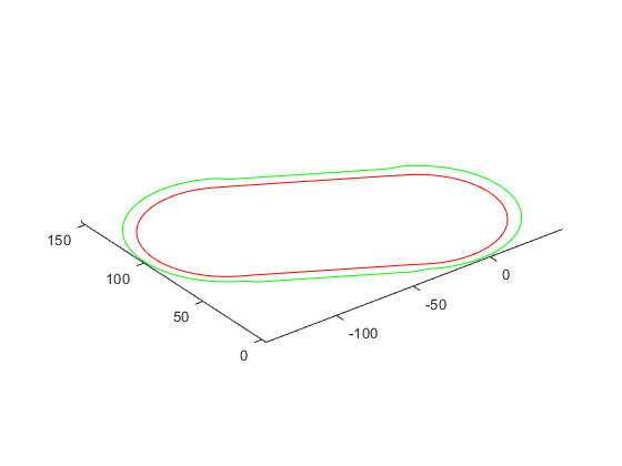
Next, call the roadBoundaries function on the vehicle and plot it as before. It will be rendered relative to the vehicle's coordinates:
figure

rb = roadBoundaries(egoCar)
outerBoundary = rb{1};
innerBoundary = rb{2};

plot3(innerBoundary(:,1),innerBoundary(:,2),innerBoundary(:,3),'r', ...
      outerBoundary(:,1),outerBoundary(:,2),outerBoundary(:,3),'g')
axis equal
rb =

  1×2 cell array

    {258×3 double}    {258×3 double}
Specify Actor Trajectory
You can position and plot any specific actor along a predefined three-dimensional path.
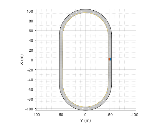
Here is an example for two vehicles that follow the racetrack at 30 m/s and 50 m/s respectively, each in its own respective lane. We offset the cars from the center of the road by setting the offset position by half a lane width of 2.7 meters, and, for the banked angle sections of the track, half the vertical height on each side:
chasePlot(egoCar);
fastCar = vehicle(scenario,'ClassID',1);

d = 2.7/2;
h = .45/2;
roadOffset = [ 0  0  0  0  d  0  0  0  0  0  0 -d  0  0  0  0
              -d -d -d -d  0  d  d  d  d  d  d  0 -d -d -d -d
               0  0  h  h  h  h  h  0  0  h  h  h  h  h  0  0]';

rWayPoints = roadCenters + roadOffset;
lWayPoints = roadCenters - roadOffset;

% loop around the track four times
rWayPoints = [repmat(rWayPoints(1:end-1,:),5,1); rWayPoints(1,:)];
lWayPoints = [repmat(lWayPoints(1:end-1,:),5,1); lWayPoints(1,:)];

smoothTrajectory(egoCar,rWayPoints(:,:), 30);
smoothTrajectory(fastCar,lWayPoints(:,:), 50);
Advance the Simulation
Actors that follow a trajectory are updated by calling advance on the driving scenario. When advance is called, each actor that is following a trajectory will move forward, and the corresponding plots will be updated. Only actors that have defined trajectories actually update. This is so you can provide your own logic while the simulation is running.
The SampleTime property in the scenario governs the interval of time between updates. By default it is 10 milliseconds, but you may specify it with arbitrary resolution:
scenario.SampleTime = 0.02
scenario =

  drivingScenario with properties:

        SampleTime: 0.0200
          StopTime: Inf
    SimulationTime: 0
         IsRunning: 1
            Actors: [1×2 driving.scenario.Vehicle]
          Barriers: [0×0 driving.scenario.Barrier]
       ParkingLots: [0×0 driving.scenario.ParkingLot]
You can run the simulation by calling advance in the conditional of a while loop and placing commands to inspect or modify the scenario within the body of the loop.
The while loop will automatically terminate when the trajectory for any vehicle has finished or an optional StopTime has been reached.
scenario.StopTime = 4;
while advance(scenario)
  pause(0.001)
end
Record a Scenario
As a convenience when the trajectories of all actors are known in advance, you can call the record function on the scenario to return a structure that contains the pose information of each actor at each time-step.
For example, you can inspect the pose information of each actor for the first 100 milliseconds of the simulation, and inspect the fifth recorded sample:
close all

scenario.StopTime = 0.100;
poseRecord = record(scenario)

r = poseRecord(5)
r.ActorPoses(1)
r.ActorPoses(2)
poseRecord =

  1×5 struct array with fields:

    SimulationTime
    ActorPoses


r =

  struct with fields:

    SimulationTime: 0.0800
        ActorPoses: [2×1 struct]


ans =

  struct with fields:

            ActorID: 1
           Position: [2.4000 -51.3502 0]
           Velocity: [30.0000 -0.0038 0]
               Roll: 0
              Pitch: 0
                Yaw: -0.0073
    AngularVelocity: [0 0 -0.0823]


ans =

  struct with fields:

            ActorID: 2
           Position: [4.0000 -48.6504 0]
           Velocity: [50.0000 -0.0105 0]
               Roll: 0
              Pitch: 0
                Yaw: -0.0120
    AngularVelocity: [0 0 -0.1235]
Incorporating Multiple Views with the Bird's Eye Plot
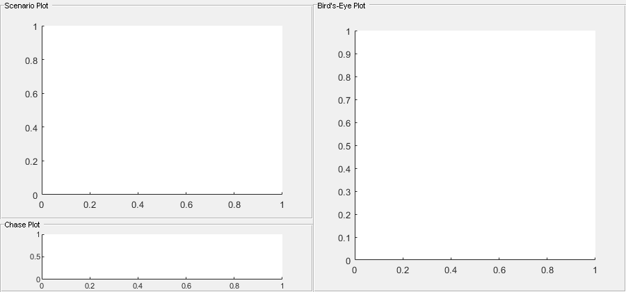
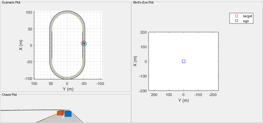
When debugging the simulation, you may wish to report the "ground truth" data in the bird's-eye plot of a specific actor while simultaneously viewing the plots generated by the scenario. To do this, you can first create a figure with axes placed in a custom arrangement:
close all;
hFigure = figure;
hFigure.Position(3) = 900;

hPanel1 = uipanel(hFigure,'Units','Normalized','Position',[0 1/4 1/2 3/4],'Title','Scenario Plot');
hPanel2 = uipanel(hFigure,'Units','Normalized','Position',[0 0 1/2 1/4],'Title','Chase Plot');
hPanel3 = uipanel(hFigure,'Units','Normalized','Position',[1/2 0 1/2 1],'Title','Bird''s-Eye Plot');

hAxes1 = axes('Parent',hPanel1);
hAxes2 = axes('Parent',hPanel2);
hAxes3 = axes('Parent',hPanel3);
Once you have the axes defined, you specify them via the Parent property when creating the plots:
% assign scenario plot to first axes and add indicators for ActorIDs 1 and 2
plot(scenario, 'Parent', hAxes1,'ActorIndicators',[1 2]);

% assign chase plot to second axes
chasePlot(egoCar, 'Parent', hAxes2);

% assign bird's-eye plot to third axes
egoCarBEP = birdsEyePlot('Parent',hAxes3,'XLimits',[-200 200],'YLimits',[-240 240]);
fastTrackPlotter = trackPlotter(egoCarBEP,'MarkerEdgeColor','red','DisplayName','target','VelocityScaling',.5);
egoTrackPlotter = trackPlotter(egoCarBEP,'MarkerEdgeColor','blue','DisplayName','ego','VelocityScaling',.5);
egoLanePlotter = laneBoundaryPlotter(egoCarBEP);
plotTrack(egoTrackPlotter, [0 0]);
egoOutlinePlotter = outlinePlotter(egoCarBEP);
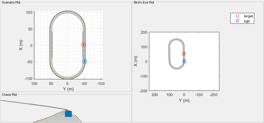
You now can restart the simulation and run it to completion, this time extracting the positional information of the target car via targetPoses and display it in the bird's-eye plot. Similarly, you can also call roadBoundaries and targetOutlines directly from the ego vehicle to extract the road boundaries and the outlines of the actors. The bird's-eye plot is capable of displaying the results of these functions directly:
restart(scenario)
scenario.StopTime = Inf;

while advance(scenario)
    t = targetPoses(egoCar);
    plotTrack(fastTrackPlotter, t.Position, t.Velocity);
    rbs = roadBoundaries(egoCar);
    plotLaneBoundary(egoLanePlotter, rbs);
    [position, yaw, length, width, originOffset, color] = targetOutlines(egoCar);
    plotOutline(egoOutlinePlotter, position, yaw, length, width, 'OriginOffset', originOffset, 'Color', color);
end
Next Steps
This example showed how to generate and visualize ground truth for synthetic sensor data and tracking algorithms using a drivingScenario object. To simulate, visualize, or modify this driving scenario in an interactive environment, try importing the drivingScenario object into the Driving Scenario Designer app:
drivingScenarioDesigner(scenario)
Further Information
For more information on how to define actors and roads, see Create Actor and Vehicle Trajectories Programmatically and Define Road Layouts Programmatically.
For a more in-depth example on how to use the bird's-eye plot with detections and tracks, see Visualize Sensor Coverage, Detections, and Tracks.
For examples that use the driving scenario to assist in generating synthetic data, see Model Radar Sensor Detections, Model Vision Sensor Detections, and Sensor Fusion Using Synthetic Radar and Vision Data.
See Also
Apps
Objects
Functions
vehicle|actorPoses|targetPoses|road|roadBoundaries|updatePlots|chasePlot|record