Create Actor and Vehicle Trajectories Programmatically
This example shows how to programmatically create actor and vehicle trajectories for a driving scenario using Automated Driving Toolbox™ functions. To create actor and vehicle trajectories interactively, use the Driving Scenario Designer app.
Actors and Vehicles
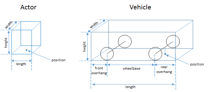
Actors in a driving scenario are defined as cuboid objects with a specific length, width, and height. Actors also have a radar cross section (specified in dBsm) which you can refine by defining angular coordinates (azimuth and elevation). Cuboid driving scenarios define the position of an actor as the center of its bottom face. Driving scenarios use this point as the point of contact of the actor with the ground. This point is also the rotational center of the actor.
A vehicle is a special kind of actor that moves on wheels. Vehicles possess three extra properties that govern the placement of the front and rear axle.
The wheelbase is the distance between the front and rear axles.
The front overhang is the amount of distance between the front axle and the front of the vehicle.
The rear overhang is the distance between the rear axle and the rear of the vehicle.
Unlike actors, the position of a vehicle is on the ground at the center of the rear axle. This position corresponds to the natural center of rotation of the vehicle.
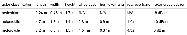
This table shows a typical list of actors and their corresponding dimensions:
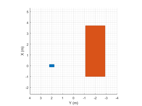
This code plots the position of an actor, with the dimensions of a typical human, and a vehicle in a driving scenario. The actor and vehicle are located at positions (0, 2) and (0, –2), respectively.
scenario = drivingScenario;
a = actor(scenario,'ClassID',1,'Length',0.24,'Width',0.45,'Height',1.7);
passingCar = vehicle(scenario,'ClassID',1);
a.Position = [0 2 0]
passingCar.Position = [0 -2 0]
plot(scenario)
ylim([-4 4])
Warning: Class ID 1 is not supported for an actor. The drivingScenario object
created a vehicle instead. ClassID of actor must be one of these values: 3
(Bicycle), 4 (Pedestrian), 5 (Jersey Barrier), or 6 (Guardrail).

a =

  Vehicle with properties:

         FrontOverhang: -3.5600
          RearOverhang: 1
             Wheelbase: 2.8000
             EntryTime: 0
              ExitTime: Inf
               ActorID: 1
               ClassID: 1
                  Name: ""
             AssetType: "Unspecified"
             AssetPath: ""
             PlotColor: [0.0660 0.4430 0.7450]
              Position: [0 2 0]
              Velocity: [0 0 0]
                   Yaw: 0
                 Pitch: 0
                  Roll: 0
       AngularVelocity: [0 0 0]
                Length: 0.2400
                 Width: 0.4500
                Height: 1.7000
                  Mesh: [1×1 extendedObjectMesh]
            RCSPattern: [2×2 double]
      RCSAzimuthAngles: [-180 180]
    RCSElevationAngles: [-90 90]


passingCar =

  Vehicle with properties:

         FrontOverhang: 0.9000
          RearOverhang: 1
             Wheelbase: 2.8000
             EntryTime: 0
              ExitTime: Inf
               ActorID: 2
               ClassID: 1
                  Name: ""
             AssetType: "Unspecified"
             AssetPath: ""
             PlotColor: [0.8660 0.3290 0]
              Position: [0 -2 0]
              Velocity: [0 0 0]
                   Yaw: 0
                 Pitch: 0
                  Roll: 0
       AngularVelocity: [0 0 0]
                Length: 4.7000
                 Width: 1.8000
                Height: 1.4000
                  Mesh: [1×1 extendedObjectMesh]
            RCSPattern: [2×2 double]
      RCSAzimuthAngles: [-180 180]
    RCSElevationAngles: [-90 90]
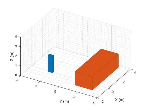
By default, the scenario plot shows an overhead view of the actors. To change this view, you can manipulate the scenario plot interactively by selecting the Camera Toolbar available in the View menu of the plot. Alternatively, you can programmatically manipulate the plot by using functions such as xlim, ylim, zlim, and view. These functions enable you to compare the relative heights of the actors.
zlim([0 4])
view(-60,30)
Define Trajectories
By using the smoothTrajectory function, you can specify actors and vehicles to follow a path along a set of waypoints at a set of given speeds. When you specify the waypoints, the smoothTrajectory function fits a piecewise clothoid curve to each segment between waypoints, preserving curvature between points. Clothoid curves have a curvature that varies linearly with distance traveled, which creates a very simple trajectory for drivers to navigate when traveling at constant velocity.
By default, actor trajectories have no curvature at the endpoints. To complete a loop, specify identical first and last waypoints.
To follow the entire trajectory at a constant speed, specify the speed as a scalar value.
Vehicles pass through the curve between waypoints at their rotational centers. Therefore, to accommodate the length of the vehicle in front of and behind the rear axle during simulation, you can offset the beginning and ending waypoints. Offsetting these waypoints fits the vehicle completely within the road at its endpoints.
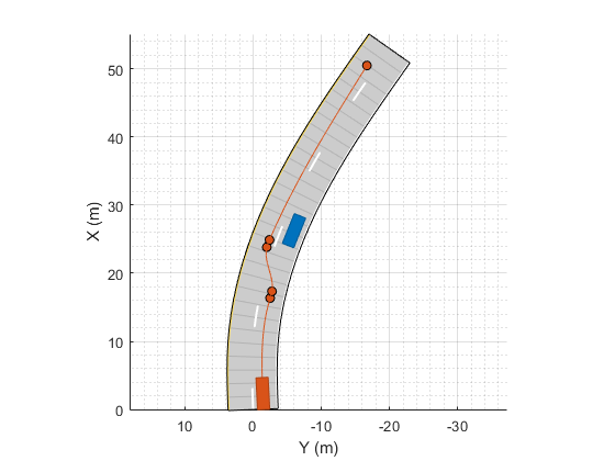
If the vehicle needs to turn quickly to avoid an obstacle, place two points close together in the intended direction of travel. This example shows a vehicle turning quickly at two places, but otherwise steering normally.
scenario = drivingScenario;
road(scenario, [0 0; 10 0; 53 -20],'lanes',lanespec(2));
plot(scenario,'Waypoints','on')
idleCar = vehicle(scenario,'ClassID',1,'Position',[25 -5.5 0],'Yaw',-22);

passingCar = vehicle(scenario,'ClassID',1)

waypoints = [1 -1.5; 16.36 -2.5; 17.35 -2.765; 23.83 -2.01; 24.9 -2.4; 50.5 -16.7];
speed = 15;
smoothTrajectory(passingCar,waypoints,speed)
passingCar =

  Vehicle with properties:

         FrontOverhang: 0.9000
          RearOverhang: 1
             Wheelbase: 2.8000
             EntryTime: 0
              ExitTime: Inf
               ActorID: 2
               ClassID: 1
                  Name: ""
             AssetType: "Unspecified"
             AssetPath: ""
             PlotColor: [0.8660 0.3290 0]
              Position: [0 0 0]
              Velocity: [0 0 0]
                   Yaw: 0
                 Pitch: 0
                  Roll: 0
       AngularVelocity: [0 0 0]
                Length: 4.7000
                 Width: 1.8000
                Height: 1.4000
                  Mesh: [1×1 extendedObjectMesh]
            RCSPattern: [2×2 double]
      RCSAzimuthAngles: [-180 180]
    RCSElevationAngles: [-90 90]
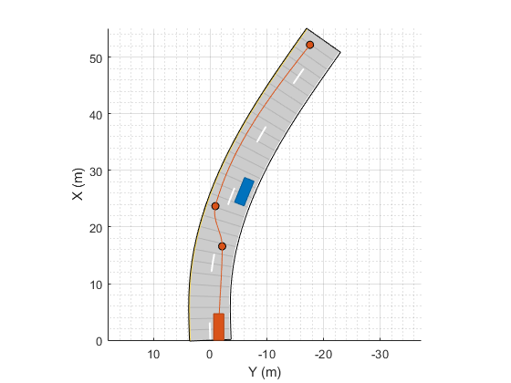
Alternatively, you can use fewer waypoints at such turns by explicitly setting the yaw orientation angle of the vehicle at each waypoint. Yaw is positive in the counterclockwise direction, and its units are in degrees. In this variation of the previous example, the trajectory is constrained such that the vehicle is at a –15 degree angle after moving into the left lane. By setting a waypoint to NaN, the smoothTrajectory function defaults to fitting a clothoid curve to the segment leading up that waypoint. In this case, that segment is the final one in the trajectory.
waypoints = [1 -1.5; 16.6 -2.1; 23.7 -0.9; 52.2 -17.6];
yaw =  [0; 0; -15; NaN];
smoothTrajectory(passingCar,waypoints,speed,'Yaw',yaw)
Turning and Braking at Intersections
For sharp turns, either define waypoints close together at the start and end of the turn or explicitly set the yaw of the vehicle at each waypoint. This setting faithfully renders the sudden change in steering.
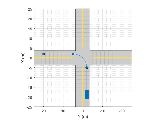
In this example, a vehicle makes a sharp left turn at an intersection using explicitly set yaw values. At the first waypoint and the waypoint before the turn, the vehicle has a yaw of 0 degrees. At the waypoint after the turn and the final waypoint, the vehicle has a yaw of 90 degrees, which is the orientation of the vehicle after completing the turn. By constraining the trajectory such that the vehicle achieves these yaw orientations, the vehicle turn is much sharper than if you had used the default yaw orientations.
The smoothTrajectory function generates a smooth, jerk-limited trajectory, with no discontinuities in acceleration between waypoints. When varying vehicle speeds, such as by slowing down at a turn, the distances between waypoints must be great enough for the vehicle to reach the desired speed while maintaining smooth acceleration throughout. Alternatively, at shorter distances, the changes in speeds must be relatively small. In this example, the vehicle decelerates from a speed of 6 m/s to 5 m/s as it enters the turn. After completing the turn, the vehicle accelerates back to its original speed.
scenario = drivingScenario;
road(scenario,[0 -25; 0 25],'lanes',lanespec([1 1]));
road(scenario,[-25 0; 25 0],'lanes',lanespec([1 1]));

turningCar = vehicle(scenario,'ClassID',1);

waypoints = [-20 -2; -5 -2; 2 5; 2 20];
speed = [6 5 5 6];
yaw = [0 0 90 90];
smoothTrajectory(turningCar,waypoints,speed,'Yaw',yaw)

plot(scenario,'Waypoints','on')
Move Vehicles
After you define all the roads, actors, and actor trajectories, you can increment the position of each actor by using the advance function on the driving scenario in a loop.
while advance(scenario)
    pause(0.01)
end
Move Vehicles in Reverse
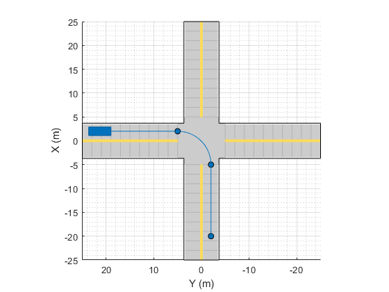
To specify reverse driving motions, specify a trajectory with negative speeds. When switching between forward and reverse motions, you must specify a waypoint between these motions that has a speed of 0. At this waypoint, the vehicle decelerates until it comes to a complete stop, and then changes driving directions.
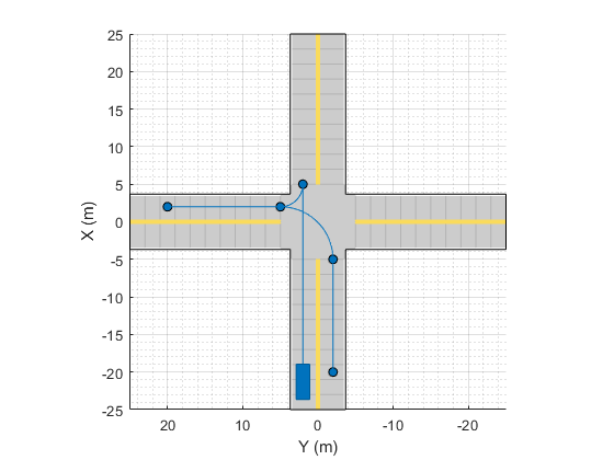
This example expands on the previous example. This time, after completing the left turn, the vehicle backs up and reverses at the intersection. Then, the vehicle switches direction again and drives forward until it stops in the opposite lane from where it started. Because the vehicle travels at slow speeds, to speed up the simulation, specify a shorter pause between simulation updates.
scenario = drivingScenario;
road(scenario,[0 -25; 0 25],'lanes',lanespec([1 1]));
road(scenario,[-25 0; 25 0],'lanes',lanespec([1 1]));

turningCar = vehicle(scenario,'ClassID',1);

waypoints = [-20 -2; -5 -2; 2 5; 2 20; 2 5; 5 2; -20 2];
speed = [6 5 5 0 -2 0 5];
yaw =  [0 0 90 90 -90 0 -180];
smoothTrajectory(turningCar,waypoints,speed,'Yaw',yaw)

plot(scenario,'Waypoints','on')

while advance(scenario)
    pause(0.001)
end
Next Steps
This example showed how to create actor and vehicle trajectories for a driving scenario using a drivingScenario object. To simulate, visualize, or modify this driving scenario in an interactive environment, try importing the drivingScenario object into the Driving Scenario Designer app by using this command:
drivingScenarioDesigner(scenario)
See Also
Apps
Objects
Functions
actor|vehicle|road|trajectory