chasePlot
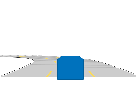
Ego-centric projective perspective plot
Description
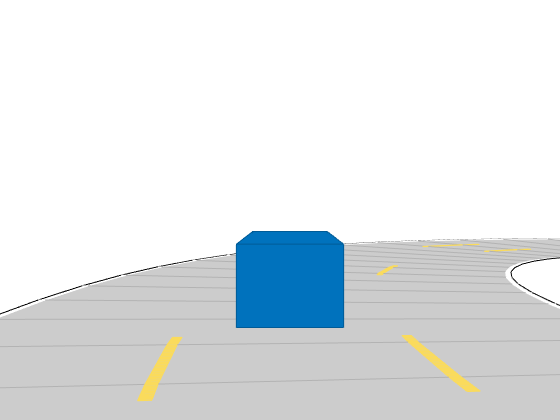
chasePlot( plots a driving scenario
from the perspective of actor ac)ac. This plot is called a
chase plot and has an ego-centric projective perspective,
where the view is positioned immediately behind the actor.
chasePlot(
specifies options using one or more name-value pairs. For example, you can display
road centers and actor waypoints on the plot.ac,Name,Value)
Examples
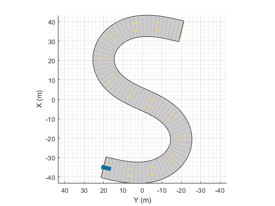
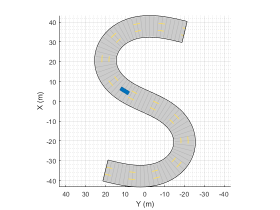
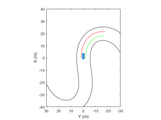
Simulate a driving scenario with one car traveling on an S-curve. Create and plot the lane boundaries.
Create the driving scenario with one road having an S-curve.
scenario = drivingScenario('StopTime',3);
roadcenters = [-35 20 0; -20 -20 0; 0 0 0; 20 20 0; 35 -20 0];
Create the lanes and add them to the road.
lm = [laneMarking('Solid','Color','w'); ...
    laneMarking('Dashed','Color','y'); ...
    laneMarking('Dashed','Color','y'); ...
    laneMarking('Solid','Color','w')];
ls = lanespec(3,'Marking',lm);
road(scenario,roadcenters,'Lanes',ls);
Add an ego vehicle and specify its trajectory from its waypoints. By default, the car travels at a speed of 30 meters per second.
car = vehicle(scenario, ...
    'ClassID',1, ...
    'Position',[-35 20 0]);
waypoints = [-35 20 0; -20 -20 0; 0 0 0; 20 20 0; 35 -20 0];
smoothTrajectory(car,waypoints);
Plot the scenario and corresponding chase plot.
plot(scenario)
chasePlot(car)
Run the simulation loop.
Initialize a bird's-eye plot and create an outline plotter, left-lane and right-lane boundary plotters, and a road boundary plotter.
Obtain the road boundaries and rectangular outlines.
Obtain the lane boundaries to the left and right of the vehicle.
Advance the simulation and update the plotters.
bep = birdsEyePlot('XLim',[-40 40],'YLim',[-30 30]);
olPlotter = outlinePlotter(bep);
lblPlotter = laneBoundaryPlotter(bep,'Color','r','LineStyle','-');
lbrPlotter = laneBoundaryPlotter(bep,'Color','g','LineStyle','-');
rbsEdgePlotter = laneBoundaryPlotter(bep);
legend('off');
while advance(scenario)
    rbs = roadBoundaries(car);
    [position,yaw,length,width,originOffset,color] = targetOutlines(car);
    lb = laneBoundaries(car,'XDistance',0:5:30,'LocationType','Center', ...
        'AllBoundaries',false);
    plotLaneBoundary(rbsEdgePlotter,rbs)
    plotLaneBoundary(lblPlotter,{lb(1).Coordinates})
    plotLaneBoundary(lbrPlotter,{lb(2).Coordinates})
    plotOutline(olPlotter,position,yaw,length,width, ...
        'OriginOffset',originOffset,'Color',color)
end
Create a driving scenario and show how target outlines change as the simulation advances.
Create a driving scenario consisting of two intersecting straight roads. The first road segment is 45 meters long. The second straight road is 32 meters long with jersey barriers along both its edges, and intersects the first road. A car traveling at 12.0 meters per second along the first road approaches a running pedestrian crossing the intersection at 2.0 meters per second.
scenario = drivingScenario('SampleTime',0.1,'StopTime',1);
road1 = road(scenario,[-10 0 0; 45 -20 0]);
road2 = road(scenario,[-10 -10 0; 35 10 0]);
barrier(scenario,road1)
barrier(scenario,road1,'RoadEdge','left')
ped = actor(scenario,'ClassID',4,'Length',0.4,'Width',0.6,'Height',1.7);
car = vehicle(scenario,'ClassID',1);
pedspeed = 2.0;
carspeed = 12.0;
smoothTrajectory(ped,[15 -3 0; 15 3 0],pedspeed);
smoothTrajectory(car,[-10 -10 0; 35 10 0],carspeed);
Create an ego-centric chase plot for the vehicle.
chasePlot(car,'Centerline','on')

Create an empty bird's-eye plot and add an outline plotter and lane boundary plotter. Then, run the simulation. At each simulation step:
Update the chase plot to display the road boundaries and target outlines.
Update the bird's-eye plot to display the updated road boundaries and target outlines. The plot perspective is always with respect to the ego vehicle.
bepPlot = birdsEyePlot('XLim',[-50 50],'YLim',[-40 40]);
outlineplotter = outlinePlotter(bepPlot);
laneplotter = laneBoundaryPlotter(bepPlot);
legend('off')

while advance(scenario)
    rb = roadBoundaries(car);
    [position,yaw,length,width,originOffset,color] = targetOutlines(car);
    [bposition,byaw,blength,bwidth,boriginOffset,bcolor,barrierSegments] = targetOutlines(car,'Barriers');
    plotLaneBoundary(laneplotter,rb)
    plotOutline(outlineplotter,position,yaw,length,width, ...
        'OriginOffset',originOffset,'Color',color)
    plotBarrierOutline(outlineplotter,barrierSegments,bposition,byaw,blength,bwidth, ...
        'OriginOffset',boriginOffset,'Color',bcolor)
    pause(0.01)
end


Input Arguments
Actor belonging to a drivingScenario object, specified as an
Actor or Vehicle object. To create these objects, use the
actor and vehicle functions, respectively.
Name-Value Arguments
Specify optional pairs of arguments as
Name1=Value1,...,NameN=ValueN, where Name is
the argument name and Value is the corresponding value.
Name-value arguments must appear after other arguments, but the order of the
pairs does not matter.
Before R2021a, use commas to separate each name and value, and enclose
Name in quotes.
Example: chasePlot(ac,'Centerline','on','RoadCenters,'on')
displays the center line and road centers of each road segment.
Axes in which to draw the plot, specified as the comma-separated pair consisting of
'Parent' and an Axes object. If you do not
specify Parent, a new figure is created.
Display the center line of roads, specified as the comma-separated pair consisting of
'Centerline' and 'off' or
'on'. The center line follows the middle of each road
segment. Center lines are discontinuous through areas such as intersections or road
splits.
Display road centers, specified as the comma-separated pair consisting of
'RoadCenters' and 'off' or
'on'. The road centers define the roads shown in the
plot.
Display actor waypoints, specified as the comma-separated pair consisting of
'Waypoints' and 'off' or
'on'. Waypoints define the trajectory of the actor.
Display actor meshes instead of cuboids, specified as the comma-separated pair
consisting of 'Meshes' and 'off' or
'on'.
Height of the plot viewpoint, specified as the comma-separated pair
consisting of 'ViewHeight' and a positive real
scalar. The height is with respect to the bottom of the actor. Units are
in meters.
Location of the plot viewpoint, specified as the comma-separated pair
consisting of 'ViewLocation' and an
[x, y] real-valued vector. The
location is with respect to the cuboid center in the coordinate system
of the actor. The default location of the viewpoint is behind the cuboid
center, [2.5*actor.Length 0]. Units are in
meters.
Roll angle orientation of the plot viewpoint, specified as the
comma-separated pair consisting of 'ViewRoll' and a
real scalar. Units are in degrees.
Pitch angle orientation of the plot viewpoint, specified as the
comma-separated pair consisting of 'ViewPitch' and a
real scalar. Units are in degrees.
Yaw angle orientation of the plot viewpoint, specified as the
comma-separated pair consisting of 'ViewYaw' and a
real scalar. Units are in degrees.
Version History
Introduced in R2017a
MATLAB Command
You clicked a link that corresponds to this MATLAB command:
Run the command by entering it in the MATLAB Command Window. Web browsers do not support MATLAB commands.
Website auswählen
Wählen Sie eine Website aus, um übersetzte Inhalte (sofern verfügbar) sowie lokale Veranstaltungen und Angebote anzuzeigen. Auf der Grundlage Ihres Standorts empfehlen wir Ihnen die folgende Auswahl: .
Sie können auch eine Website aus der folgenden Liste auswählen:
So erhalten Sie die bestmögliche Leistung auf der Website
Wählen Sie für die bestmögliche Website-Leistung die Website für China (auf Chinesisch oder Englisch). Andere landesspezifische Websites von MathWorks sind für Besuche von Ihrem Standort aus nicht optimiert.
Amerika
- América Latina (Español)
- Canada (English)
- United States (English)
Europa
- Belgium (English)
- Denmark (English)
- Deutschland (Deutsch)
- España (Español)
- Finland (English)
- France (Français)
- Ireland (English)
- Italia (Italiano)
- Luxembourg (English)
- Netherlands (English)
- Norway (English)
- Österreich (Deutsch)
- Portugal (English)
- Sweden (English)
- Switzerland
- United Kingdom (English)