Visualize Image Classifications Using Maximal and Minimal Activating Images
This example shows how to use a data set to find out what activates the channels of a deep neural network. This allows you to understand how a neural network works and diagnose potential issues with a training data set.
This example covers a number of simple visualization techniques, using a GoogLeNet transfer-learned on a food data set. By looking at images that maximally or minimally activate the classifier, you can discover why a neural network gets classifications wrong.
Load and Preprocess the Data
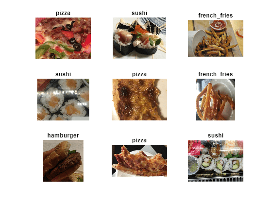
Load the images as an image datastore. This small data set contains a total of 978 observations with 9 classes of food.
Split this data into a training, validation, and test sets to prepare for transfer learning using GoogLeNet.
rng default
dataDir = fullfile(tempdir,"Food Dataset");
url = "https://www.mathworks.com/supportfiles/nnet/data/ExampleFoodImageDataset.zip";

if ~exist(dataDir,"dir")
    mkdir(dataDir);
end

downloadExampleFoodImagesData(url,dataDir);
Skipping download, file already exists...
Skipping unzipping, file already unzipped...
Done.
imds = imageDatastore(dataDir, ...
    "IncludeSubfolders",true,"LabelSource","foldernames");
[imdsTrain,imdsValidation,imdsTest] = splitEachLabel(imds,0.6,0.2);
View the class names of the training data.
classNames = categories(imdsTrain.Labels)
classNames = 9×1 cell
    {'caesar_salad' }
    {'caprese_salad'}
    {'french_fries' }
    {'greek_salad'  }
    {'hamburger'    }
    {'hot_dog'      }
    {'pizza'        }
    {'sashimi'      }
    {'sushi'        }
View the number of classes.
numClasses = numel(classNames)
numClasses = 9
Display a selection of images from the data set.
rnd = randperm(numel(imds.Files),9);
for i = 1:numel(rnd)
subplot(3,3,i)
imshow(imread(imds.Files{rnd(i)}))
label = imds.Labels(rnd(i));
title(label,"Interpreter","none")
end
Train Network to Classify Food Images
Load a pretrained GoogLeNet network and the corresponding class names. This requires the Deep Learning Toolbox™ Model for GoogLeNet Network support package. If this support package is not installed, then the software provides a download link. For a list of all available networks, see Pretrained Deep Neural Networks.
The convolutional layers of the network extract image features that the last learnable layer and the final softmax layer use to classify the input image. These two layers, 'loss3-classifier' and 'prob' in GoogLeNet, contain information on how to combine the features that the network extracts into class probabilities, a loss value, and predicted labels. To return a neural network ready for retraining for the new data, also specify the number of classes.
net = imagePretrainedNetwork("googlenet","NumClasses",numClasses);
Increase the learn rates of the new fully-connected layer.
fcLayer = net.Layers(end-1);
fcLayer.WeightLearnRateFactor = 10;
fcLayer.BiasLearnRateFactor = 10;
net = replaceLayer(net,fcLayer.Name,fcLayer);
The first element of the Layers property of the network is the image input layer. This layer requires input images of size 224-by-224-by-3, where 3 is the number of color channels.
inputSize = net.Layers(1).InputSize;
Train Network
The network requires input images of size 224-by-224-by-3, but the images in the image datastore have different sizes. Use an augmented image datastore to automatically resize the training images. Specify additional augmentation operations to perform on the training images: randomly flip the training images along the vertical axis, randomly translate them up to 30 pixels, and scale them up to 10% horizontally and vertically. Data augmentation helps prevent the network from overfitting and memorizing the exact details of the training images.
pixelRange = [-30 30];
scaleRange = [0.9 1.1];
imageAugmenter = imageDataAugmenter( ...
    'RandXReflection',true, ...
    'RandXTranslation',pixelRange, ...
    'RandYTranslation',pixelRange, ...
    'RandXScale',scaleRange, ...
    'RandYScale',scaleRange);
augimdsTrain = augmentedImageDatastore(inputSize(1:2),imdsTrain, ...
    'DataAugmentation',imageAugmenter);
To automatically resize the validation images without performing further data augmentation, use an augmented image datastore without specifying any additional preprocessing operations.
augimdsValidation = augmentedImageDatastore(inputSize(1:2),imdsValidation);
Specify the training options. Choosing among the options requires empirical analysis. To explore different training option configurations by running experiments, you can use the Experiment Manager app.
Train using the SGDM optimizer.
Set
InitialLearnRateto a small value to slow down learning in the transferred layers that are not already frozen. In the previous step, you increased the learning rate factors for the last learnable layer to speed up learning in the new final layers. This combination of learning rate settings results in fast learning in the new layers, slower learning in the middle layers, and no learning in the earlier, frozen layers.Specify the number of epochs to train for. When performing transfer learning, you do not need to train for as many epochs. An epoch is a full training cycle on the entire training data set.
Specify the mini-batch size and validation data. Compute the validation accuracy once per epoch.
Display the training progress in a plot and monitor the accuracy.
Disable the verbose output.
miniBatchSize = 10;
valFrequency = floor(numel(augimdsTrain.Files)/miniBatchSize);
options = trainingOptions('sgdm', ...
    'MiniBatchSize',miniBatchSize, ...
    'MaxEpochs',4, ...
    'InitialLearnRate',3e-4, ...
    'Shuffle','every-epoch', ...
    'ValidationData',augimdsValidation, ...
    'ValidationFrequency',valFrequency, ...
    'Plots','training-progress', ...
    'Metric',"accuracy",...
    'Verbose',false);
Train the neural network using the trainnet function. For classification, use cross-entropy loss. By default, the trainnet function uses a GPU if one is available. Training on a GPU requires a Parallel Computing Toolbox™ license and a supported GPU device. For information on supported devices, see GPU Computing Requirements (Parallel Computing Toolbox). Otherwise, the trainnet function uses the CPU. To specify the execution environment, use the ExecutionEnvironment training option. Because this data set is small, the training is fast. If you run this example and train the network yourself, you will get different results and misclassifications caused by the randomness involved in the training process.
net = trainnet(augimdsTrain,net,"crossentropy",options);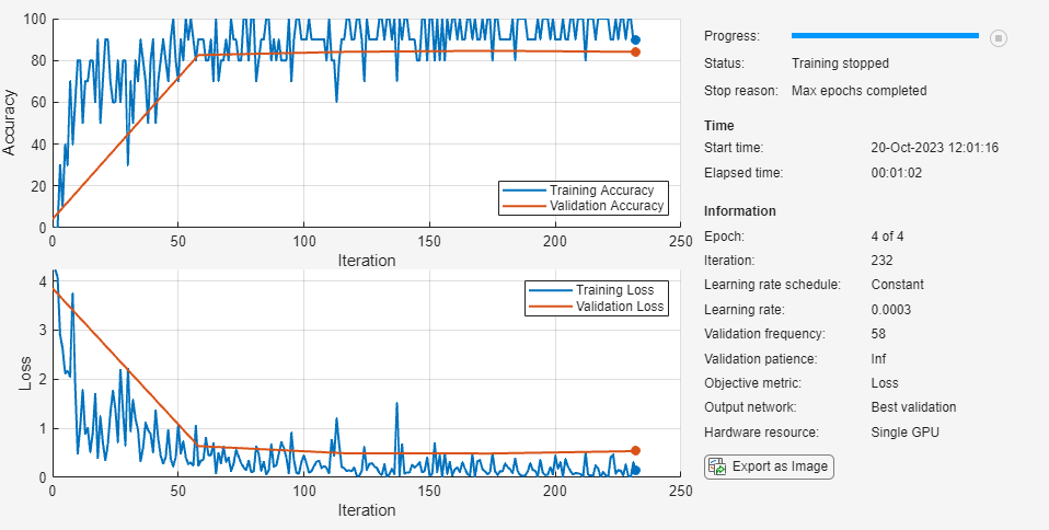
Classify Test Images
Classify the test images and calculate the classification accuracy. To make predictions with multiple observations, use the minibatchpredict function. To convert the prediction scores to labels, use the scores2label function. The minibatchpredict function automatically uses a GPU if one is available. Using a GPU requires a Parallel Computing Toolbox™ license and a supported GPU device. For information on supported devices, see GPU Computing Requirements (Parallel Computing Toolbox). Otherwise, the function uses the CPU.
augimdsTest = augmentedImageDatastore(inputSize(1:2),imdsTest);

predictedScores = minibatchpredict(net,augimdsTest);
predictedClasses = scores2label(predictedScores,classNames);

accuracy = mean(predictedClasses == imdsTest.Labels)
accuracy = 0.8980
Confusion Matrix for the Test Set
Plot a confusion matrix of the test set predictions. This highlights which particular classes cause most problems for the network.
figure;
confusionchart(imdsTest.Labels,predictedClasses,'Normalization',"row-normalized");
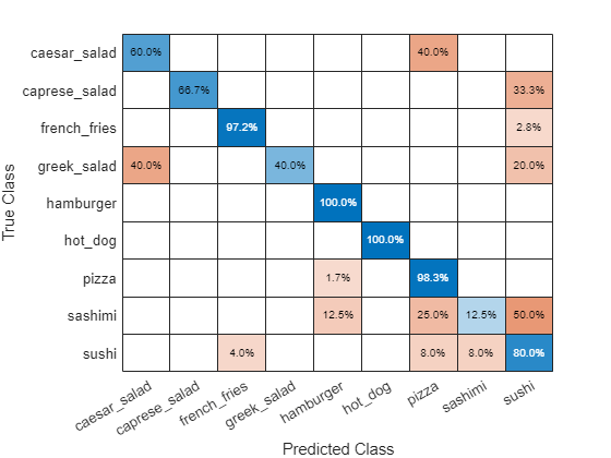
The confusion matrix shows that the network has poor performance for some classes, such as Greek salad, sashimi, hot dog, and sushi. These classes are underrepresented in the data set which may be impacting network performance. Investigate one of these classes to better understand why the network is struggling.
figure();
histogram(imdsValidation.Labels);
ax = gca();
ax.XAxis.TickLabelInterpreter = "none";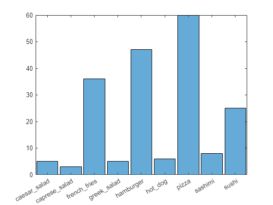
Investigate Classifications
Investigate network classification for the sushi class.
Sushi Most Like Sushi
First, find which images of sushi most strongly activate the network for the sushi class. This answers the question "Which images does the network think are most sushi-like?".
Plot the maximally-activating images, these are the input images that strongly activate the fully-connected layer's "sushi" neuron. This figure shows the top 4 images, in a descending class score.
chosenClass = "sushi";
classIdx = find(classNames == chosenClass);

numImgsToShow = 4;

[sortedScores,imgIdx] = findMaxActivatingImages(imdsTest,chosenClass,predictedScores,numImgsToShow);

figure
plotImages(imdsTest,imgIdx,sortedScores,predictedClasses,numImgsToShow)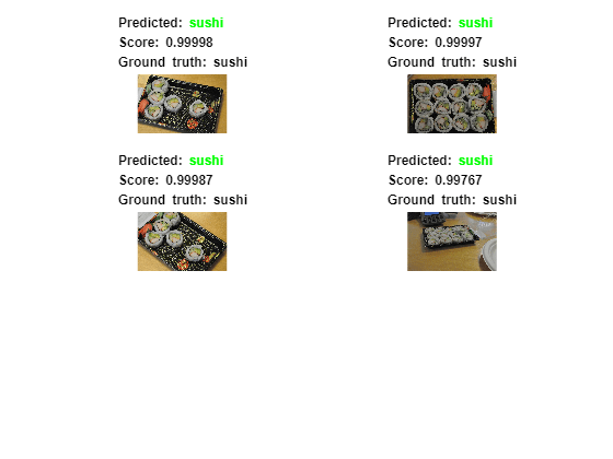
Visualize Cues for the Sushi Class
Is the network looking at the right thing for sushi? The maximally-activating images of the sushi class for the network all look similar to each other - a lot of round shapes clustered closely together.
The network is doing well at classifying those kinds of sushi. However, to verify that this is true and to better understand why the network makes its decisions, use a visualization technique like Grad-CAM. For more information on using Grad-CAM, see Grad-CAM Reveals the Why Behind Deep Learning Decisions.
Read the first resized image from the augmented image datastore, then plot the Grad-CAM visualization using gradCAM.
imageNumber = 1;

observation = augimdsTest.readByIndex(imgIdx(imageNumber));
img = observation.input{1};

label = predictedClasses(imgIdx(imageNumber));
score = sortedScores(imageNumber);

gradcamMap = gradCAM(net,img,label);

figure
alpha = 0.5;
plotGradCAM(img,gradcamMap,alpha);
sgtitle(string(label)+" (score: "+ max(score)+")")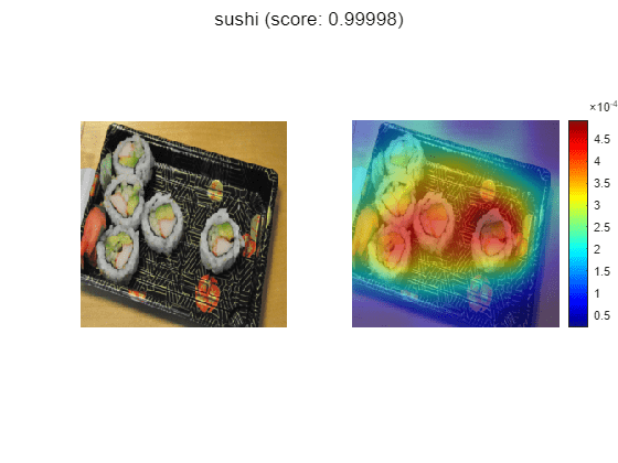
The Grad-CAM map confirms that the network is focusing on the sushi in the image. However you can also see that the network is looking at parts of the plate and the table.
Sushi Least Like Sushi
Now find which images of sushi activate the network for the sushi class the least. This answers the question "Which images does the network think are less sushi-like?". Some of these images, for example images 3 and 4 actually contain sashimi, which means the network isn't actually misclassifying them. These images are mislabeled.
This is useful because it finds the images on which the network performs badly, and it provides some insight into its decision.
chosenClass = "sushi";
numImgsToShow = 9;

[sortedScores,imgIdx] = findMinActivatingImages(imdsTest,chosenClass,predictedScores,numImgsToShow);

figure
plotImages(imdsTest,imgIdx,sortedScores,predictedClasses,numImgsToShow)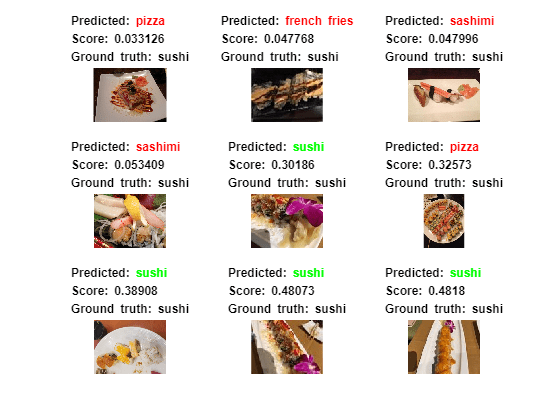
Investigate Sushi Misclassified as Sashimi
Why is the network classifying sushi incorrectly? To see what the network is focusing on, run the Grad-CAM technique on one of these images.
imageNumber = 4;
observation = augimdsTest.readByIndex(imgIdx(imageNumber));
img = observation.input{1};

label = predictedClasses(imgIdx(imageNumber));
score = sortedScores(imageNumber);

gradcamMap = gradCAM(net,img,label);

figure
alpha = 0.5;
plotGradCAM(img,gradcamMap,alpha);
title(string(label)+" (sushi score: "+ max(score)+")")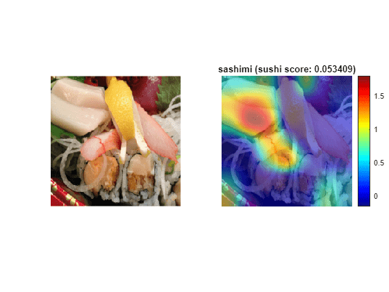
As expected, the network focuses on the sashimi instead of the sushi.
Conclusions
Investigating the datapoints that give rise to large or small class scores, and datapoints that the network classifies confidently but incorrectly, is a simple technique which can provide useful insight into how a trained network is functioning. In the case of the food data set, this example highlighted that:
The test data contains several images with incorrect true labels, such as the "sashimi" which is actually "sushi". The data also contains incomplete labels, such as images which contain both sushi and sashimi.
The network considers a "sushi" to be "multiple, clustered, round-shaped things". However, it must be able to distinguish a lone sushi as well.
To improve performance the network needs to see more images from the underrepresented classes.
Helper Functions
function downloadExampleFoodImagesData(url,dataDir)
% Download the Example Food Image data set, containing 978 images of
% different types of food split into 9 classes.

% Copyright 2019 The MathWorks, Inc.

fileName = "ExampleFoodImageDataset.zip";
fileFullPath = fullfile(dataDir,fileName);

% Download the .zip file into a temporary directory.
if ~exist(fileFullPath,"file")
    fprintf("Downloading MathWorks Example Food Image dataset...\n");
    fprintf("This can take several minutes to download...\n");
    websave(fileFullPath,url);
    fprintf("Download finished...\n");
else
    fprintf("Skipping download, file already exists...\n");
end

% Unzip the file.
%
% Check if the file has already been unzipped by checking for the presence
% of one of the class directories.
exampleFolderFullPath = fullfile(dataDir,"pizza");
if ~exist(exampleFolderFullPath,"dir")
    fprintf("Unzipping file...\n");
    unzip(fileFullPath,dataDir);
    fprintf("Unzipping finished...\n");
else
    fprintf("Skipping unzipping, file already unzipped...\n");
end
fprintf("Done.\n");

end

function [sortedScores,imgIdx] = findMaxActivatingImages(imds,className,predictedScores,numImgsToShow)
% Find the predicted scores of the chosen class on all the images of the chosen class
% (e.g. predicted scores for sushi on all the images of sushi)
[scoresForChosenClass,imgsOfClassIdxs] = findScoresForChosenClass(imds,className,predictedScores);

% Sort the scores in descending order
[sortedScores,idx] = sort(scoresForChosenClass,'descend');

% Return the indices of only the first few
imgIdx = imgsOfClassIdxs(idx(1:numImgsToShow));

end

function [sortedScores,imgIdx] = findMinActivatingImages(imds,className,predictedScores,numImgsToShow)
% Find the predicted scores of the chosen class on all the images of the chosen class
% (e.g. predicted scores for sushi on all the images of sushi)
[scoresForChosenClass,imgsOfClassIdxs] = findScoresForChosenClass(imds,className,predictedScores);

% Sort the scores in ascending order
[sortedScores,idx] = sort(scoresForChosenClass,'ascend');

% Return the indices of only the first few
imgIdx = imgsOfClassIdxs(idx(1:numImgsToShow));

end

function [scoresForChosenClass,imgsOfClassIdxs] = findScoresForChosenClass(imds,className,predictedScores)
% Find the index of className (e.g. "sushi" is the 9th class)
uniqueClasses = unique(imds.Labels);
chosenClassIdx = string(uniqueClasses) == className;

% Find the indices in imageDatastore that are images of label "className"
% (e.g. find all images of class sushi)
imgsOfClassIdxs = find(imds.Labels == className);

% Find the predicted scores of the chosen class on all the images of the
% chosen class
% (e.g. predicted scores for sushi on all the images of sushi)
scoresForChosenClass = predictedScores(imgsOfClassIdxs,chosenClassIdx);
end

function plotImages(imds,imgIdx,sortedScores,predictedClasses,numImgsToShow)

for i=1:numImgsToShow
    score = sortedScores(i);
    sortedImgIdx = imgIdx(i);
    predClass = predictedClasses(sortedImgIdx);
    correctClass = imds.Labels(sortedImgIdx);

    imgPath = imds.Files{sortedImgIdx};

    if predClass == correctClass
        color = "\color{green}";
    else
        color = "\color{red}";
    end

    predClassTitle = strrep(string(predClass),'_',' ');
    correctClassTitle = strrep(string(correctClass),'_',' ');

    subplot(3,ceil(numImgsToShow./3),i)
    imshow(imread(imgPath));
    title("Predicted: " + color + predClassTitle + "\newline\color{black}Score: " + num2str(score) + "\newlineGround truth: " + correctClassTitle);
end

end

function plotGradCAM(img,gradcamMap,alpha)

subplot(1,2,1)
imshow(img);

h = subplot(1,2,2);
imshow(img)
hold on;
imagesc(gradcamMap,'AlphaData',alpha);

originalSize2 = get(h,'Position');

colormap jet
colorbar

set(h,'Position',originalSize2);
hold off;
end
See Also
imagePretrainedNetwork | dlnetwork | trainingOptions | trainnet | testnet | imageDatastore | augmentedImageDatastore | confusionchart | minibatchpredict | scores2label | occlusionSensitivity | gradCAM | imageLIME