Train Deep Learning Semantic Segmentation Network Using 3-D Simulation Data
This example shows how to use 3-D simulation data to train a semantic segmentation network and fine-tune it to real-world data using generative adversarial networks (GANs).
This example uses 3-D simulation data generated by Driving Scenario Designer and the Unreal Engine®. For an example showing how to generate such simulation data, see Depth and Semantic Segmentation Visualization Using Unreal Engine Simulation (Automated Driving Toolbox). The 3-D simulation environment generates the images and the corresponding ground truth pixel labels. Using the simulation data avoids the annotation process, which is both tedious and requires a large amount of human effort. However, domain shift models trained on only simulation data do not perform well on real-world data sets. To address this, you can use domain adaptation to fine-tune the trained model to work on a real-world data set.
This example uses AdaptSegNet [1], a network that adapts the structure of the output segmentation predictions, which look alike irrespective of the input domain. The AdaptSegNet network is based on the GAN model and consists of two networks that are trained simultaneously to maximize the performance of both:
Generator — Network trained to generate high-quality segmentation results from real or simulated input images
Discriminator — Network that compares and attempts to distinguish whether the segmentation predictions of the generator are from real or simulated data
To fine-tune the AdaptSegNet model for real-world data, this example uses a subset of the CamVid data [2] and adapts the model to generate high-quality segmentation predictions on the CamVid data.
Download Pretrained Network
Download the pretrained network. The pretrained model allows you to run the entire example without having to wait for training to complete. If you want to train the network, set the doTraining variable to true.
doTraining = false;
if ~doTraining
    pretrainedURL = 'https://ssd.mathworks.com/supportfiles/vision/data/trainedAdaptSegGANNet.mat';
    pretrainedFolder = fullfile(tempdir,'pretrainedNetwork');
    pretrainedNetwork = fullfile(pretrainedFolder,'trainedAdaptSegGANNet.mat');
    if ~exist(pretrainedNetwork,'file')
        mkdir(pretrainedFolder);
        disp('Downloading pretrained network (57 MB)...');
        websave(pretrainedNetwork,pretrainedURL);
    end
    pretrained = load(pretrainedNetwork);
end
Download Data Sets
Download the simulation and real data sets by using the downloadDataset function, defined in the Supporting Functions section of this example. The downloadDataset function downloads the entire CamVid data set and partition the data into training and test sets.
The simulation data set was generated by Driving Scenario Designer. The generated scenarios, which consist of 553 photorealistic images with labels, were rendered by the Unreal Engine. You use this data set to train the model.
The real data set is a subset of the CamVid data set from the University of Cambridge. To adapt the model to real-world data, 69 CamVid images. To evaluate the trained model, you use 368 CamVid images.
The download time depends on your internet connection.
simulationDataURL = 'https://ssd.mathworks.com/supportfiles/vision/data/SimulationDrivingDataset.zip';
realImageDataURL = 'http://web4.cs.ucl.ac.uk/staff/g.brostow/MotionSegRecData/files/701_StillsRaw_full.zip';
realLabelDataURL = 'http://web4.cs.ucl.ac.uk/staff/g.brostow/MotionSegRecData/data/LabeledApproved_full.zip';

simulationDataLocation = fullfile(tempdir,'SimulationData');
realDataLocation = fullfile(tempdir,'RealData');
[simulationImagesFolder, simulationLabelsFolder, realImagesFolder, realLabelsFolder, ...
    realTestImagesFolder, realTestLabelsFolder] = ...
    downloadDataset(simulationDataLocation,simulationDataURL,realDataLocation,realImageDataURL,realLabelDataURL);
The downloaded files include the pixel labels for the real domain, but note that you do not use these pixel labels in the training process. This example uses the real domain pixel labels only to calculate the mean intersection over union (IoU) value to evaluate the efficacy of the trained model.
Load Simulation and Real Data
Use imageDatastore to load the simulation and real data sets for training. By using an image datastore, you can efficiently load a large collection of images on disk.
simData = imageDatastore(simulationImagesFolder);
realData = imageDatastore(realImagesFolder);
Preview images from the simulation data set and real data set.
simImage = preview(simData);
realImage = preview(realData);
montage({simImage,realImage})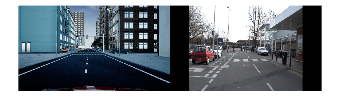
The real and simulated images look very different. Consequently, models trained on simulated data and evaluated on real data perform poorly due to domain shift.
Load Pixel-Labeled Images for Simulation Data and Real Data
Load the simulation pixel label image data by using pixelLabelDatastore (Computer Vision Toolbox). A pixel label datastore encapsulates the pixel label data and the label ID to a class name mapping.
For this example, specify five classes useful for an automated driving application: road, background, pavement, sky, and car.
classes = [
    "Road"
    "Background"
    "Pavement"
    "Sky"
    "Car"
    ];
numClasses = numel(classes);
The simulation data set has eight classes. Reduce the number of classes from eight to five by grouping the building, tree, traffic signal, and light classes from the original data set into a single background class. Return the grouped label IDs by using the helper function simulationPixelLabelIDs. This helper function is attached to the example as a supporting file.
labelIDs = simulationPixelLabelIDs;
Use the classes and label IDs to create a pixel label datastore of the simulation data.
simLabels = pixelLabelDatastore(simulationLabelsFolder,classes,labelIDs);
Initialize the colormap for the segmented images using the helper function domainAdaptationColorMap, defined in the Supporting Functions section.
dmap = domainAdaptationColorMap;
Preview a pixel-labeled image by overlaying the label on top of the image using the labeloverlay (Image Processing Toolbox) function.
simImageLabel = preview(simLabels);
overlayImageSimulation = labeloverlay(simImage,simImageLabel,'ColorMap',dmap);
figure
imshow(overlayImageSimulation)
labelColorbar(dmap,classes);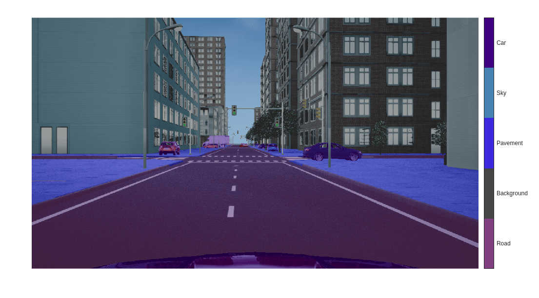
Shift the simulation and real data used for training to zero center, to center the data around the origin, by using the transform function and the preprocessData helper function, defined in the Supporting Functions section.
preprocessedSimData = transform(simData, @(simdata)preprocessData(simdata));
preprocessedRealData = transform(realData, @(realdata)preprocessData(realdata));
Use the combine function to combine the transformed image datastore and pixel label datastores of the simulation domain. The training process does not use the pixel labels of real data.
combinedSimData = combine(preprocessedSimData,simLabels);
Define AdaptSegNet Generator
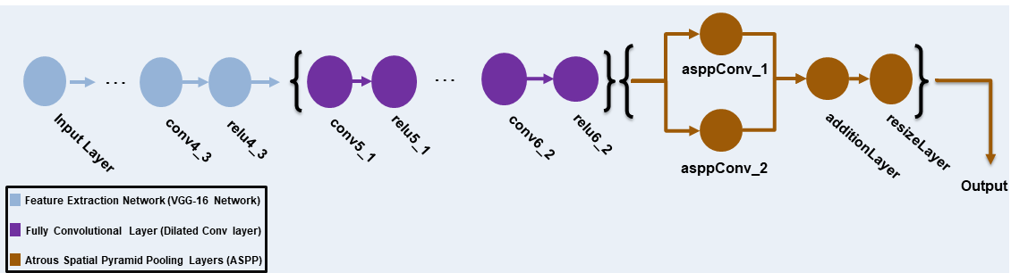
This example modifies the VGG-16 network pretrained on ImageNet to a fully convolutional network. To enlarge the receptive fields, dilated convolutional layers with strides of 2 and 4 are added. This makes the output feature map resolution one-eighth of the input size. Atrous spatial pyramid pooling (ASPP) is used to provide multiscale information and is followed by a resize2dlayer with an upsampling factor of 8 to resize the output to the size of the input.
The AdaptSegNet generator network used in this example is illustrated in the following diagram.
To get a pretrained VGG-16 network, install the vgg16. If the support package is not installed, then the software provides a download link.
[net,~] = imagePretrainedNetwork('vgg16'); To make the VGG-16 network suitable for semantic segmentation, remove all VGG layers after 'relu4_3'.
vggLayers = net.Layers(2:24);
Create an image input layer of size 1280-by-720-by-3 for the generator.
inputSizeGenerator = [1280 720 3];
inputLayer = imageInputLayer(inputSizeGenerator,'Normalization','None','Name','inputLayer');
Create fully convolutional network layers. Use dilation factors of 2 and 4 to enlarge the respective fields.
fcnlayers = [
    convolution2dLayer([3 3], 360,'DilationFactor',[2 2],'Padding',[2 2 2 2],'Name','conv5_1','WeightsInitializer','narrow-normal','BiasInitializer','zeros')
    reluLayer('Name','relu5_1')
    convolution2dLayer([3 3], 360,'DilationFactor',[2 2],'Padding',[2 2 2 2] ,'Name','conv5_2','WeightsInitializer','narrow-normal','BiasInitializer','zeros')
    reluLayer('Name','relu5_2')
    convolution2dLayer([3 3], 360,'DilationFactor',[2 2],'Padding',[2 2 2 2],'Name','conv5_3','WeightsInitializer','narrow-normal','BiasInitializer','zeros')
    reluLayer('Name','relu5_3')
    convolution2dLayer([3 3], 480,'DilationFactor',[4 4],'Padding',[4 4 4 4],'Name','conv6_1','WeightsInitializer','narrow-normal','BiasInitializer','zeros')
    reluLayer('Name','relu6_1')
    convolution2dLayer([3 3], 480,'DilationFactor',[4 4],'Padding',[4 4 4 4] ,'Name','conv6_2','WeightsInitializer','narrow-normal','BiasInitializer','zeros')
    reluLayer('Name','relu6_2')
    ];
Combine the layers and create the generator network.
layers = [
    inputLayer
    vggLayers
    fcnlayers
    ];
dlnetGenerator = dlnetwork(layers);
ASPP is used to provide multiscale information. Add the ASPP module to the generator network with a filter size equal to the number of channels by using the addASPPToNetwork helper function, defined in the Supporting Functions section.
dlnetGenerator = addASPPToNetwork(dlnetGenerator, numClasses);
Apply resize2dLayer with an upsampling factor of 8 to make the output match the size of the input.
upSampleLayer = resize2dLayer('Scale',8,'Method','bilinear','Name','resizeLayer');
dlnetGenerator = addLayers(dlnetGenerator,upSampleLayer);
dlnetGenerator = connectLayers(dlnetGenerator,'additionLayer','resizeLayer');
Visualize the generator network in a plot.
plot(dlnetGenerator)
title("Generator")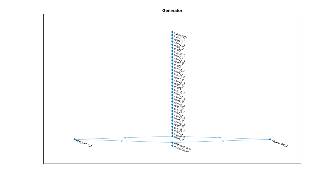
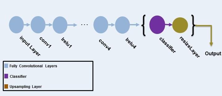
Define AdaptSeg Discriminator
The discriminator network consists of five convolutional layers with a kernel size of 3 and a stride of 2, where the number of channels is {64, 128, 256, 512, 1}. Each layer is followed by a leaky ReLU layer parameterized by a scale of 0.2, except for the last layer. resize2dLayer is used to resize the output of the discriminator. Note that this example does not use batch normalization, as the discriminator is jointly trained with the segmentation network using a small batch size.
The AdaptSegNet discriminator network in this example is illustrated in the following diagram.
Create an image input layer of size 1280-by-720-by-numClasses that takes in the segmentation predictions of the simulation and real domains.
inputSizeDiscriminator = [1280 720 numClasses];
Create fully convolutional layers and generate the discriminator network.
% Factor for number of channels in convolution layer.
numChannelsFactor = 64;

% Scale factor to resize the output of the discriminator.
resizeScale = 64;

% Scalar multiplier for leaky ReLU layers.
leakyReLUScale = 0.2;

% Create the layers of the discriminator.
layers = [
    imageInputLayer(inputSizeDiscriminator,'Normalization','none','Name','inputLayer')
    convolution2dLayer(3,numChannelsFactor,'Stride',2,'Padding',1,'Name','conv1','WeightsInitializer','narrow-normal','BiasInitializer','narrow-normal')
    leakyReluLayer(leakyReLUScale,'Name','lrelu1')
    convolution2dLayer(3,numChannelsFactor*2,'Stride',2,'Padding',1,'Name','conv2','WeightsInitializer','narrow-normal','BiasInitializer','narrow-normal')
    leakyReluLayer(leakyReLUScale,'Name','lrelu2')
    convolution2dLayer(3,numChannelsFactor*4,'Stride',2,'Padding',1,'Name','conv3','WeightsInitializer','narrow-normal','BiasInitializer','narrow-normal')
    leakyReluLayer(leakyReLUScale,'Name','lrelu3')
    convolution2dLayer(3,numChannelsFactor*8,'Stride',2,'Padding',1,'Name','conv4','WeightsInitializer','narrow-normal','BiasInitializer','narrow-normal')
    leakyReluLayer(leakyReLUScale,'Name','lrelu4')
    convolution2dLayer(3,1,'Stride',2,'Padding',1,'Name','classifer','WeightsInitializer','narrow-normal','BiasInitializer','narrow-normal')
    resize2dLayer('Scale', resizeScale,'Method','bilinear','Name','resizeLayer');
    ];

% Create the dlnetwork of the discriminator.
dlnetDiscriminator  = dlnetwork(layers);
Visualize the discriminator network in a plot.
plot(dlnetDiscriminator)
title("Discriminator")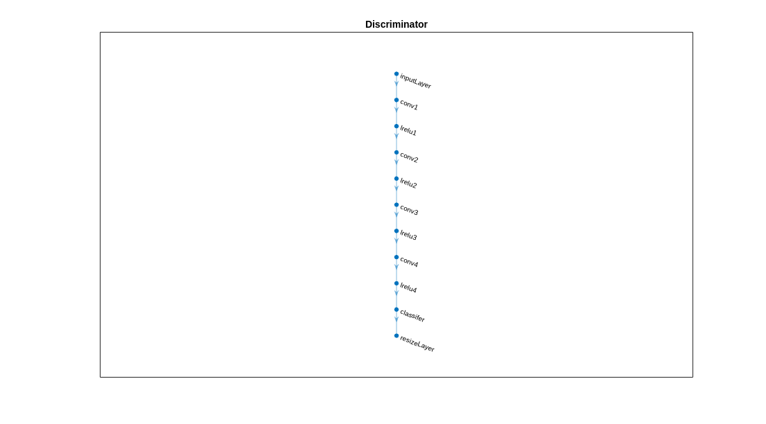
Specify Training Options
Specify these training options.
Set the total number of iterations to
5000. By doing so, you train the network for around 10 epochs.Set the learning rate for the generator to
2.5e-4.Set the learning rate for the discriminator to
1e-4.Set the L2 regularization factor to
0.0005.The learning rate exponentially decreases based on the formula . This decrease helps to stabilize the gradients at higher iterations. Set the power to
0.9.Set the weight of the adversarial loss to
0.001.Initialize the velocity of the gradient as
[ ]. This value is used by SGDM to store the velocity of the gradients.Initialize the moving average of the parameter gradients as
[ ]. This value is used by Adam initializer to store the average of parameter gradients.Initialize the moving average of squared parameter gradients as
[ ]. This value is used by Adam initializer to store the average of the squared parameter gradients.Set the mini-batch size to
1.
numIterations = 5000;
learnRateGenBase = 2.5e-4;
learnRateDisBase = 1e-4;
l2Regularization = 0.0005;
power = 0.9;
lamdaAdv = 0.001;
vel= [];
averageGrad = [];
averageSqGrad = [];
miniBatchSize = 1;
Train on a GPU, if one is available. Using a GPU requires Parallel Computing Toolbox™ and a CUDA® enabled NVIDIA® GPU. To automatically detect if you have a GPU available, set executionEnvironment to "auto". If you do not have a GPU, or do not want to use one for training, set executionEnvironment to "cpu". To ensure the use of a GPU for training, set executionEnvironment to "gpu". For information about the supported compute capabilities, see GPU Computing Requirements (Parallel Computing Toolbox).
executionEnvironment = "auto";Create the minibatchqueue object from the combined datastore of the simulation domain.
mbqTrainingDataSimulation =  minibatchqueue(combinedSimData,"MiniBatchSize",miniBatchSize, ...
    "MiniBatchFormat","SSCB","OutputEnvironment",executionEnvironment);
Create the minibatchqueue object from the input image datastore of the real domain.
mbqTrainingDataReal = minibatchqueue(preprocessedRealData,"MiniBatchSize",miniBatchSize, ...
    "MiniBatchFormat","SSCB","OutputEnvironment",executionEnvironment);
Train Model
Train the model using a custom training loop. The helper function modelGradients, defined in the Supporting Functions section of this example, calculate the gradients and losses for the generator and discriminator. Create the training progress plot using configureTrainingLossPlotter, attached to this example as a supporting file, and update the training progress using updateTrainingPlots. Loop over the training data and update the network parameters at each iteration.
For each iteration:
Read the image and label information from the
minibatchqueueobject of the simulation data using thenextfunction.Read the image information from the
minibatchqueueobject of the real data using thenextfunction.Evaluate the model gradients using
dlfevaland themodelGradientshelper function, defined in the Supporting Functions section.modelGradientsreturns the gradients of the loss with respect to the learnable parameters.Update the generator network parameters using the
sgdmupdatefunction.Update the discriminator network parameters using the
adamupdatefunction.Update the training progress plot for every iteration and display various computed losses.
if doTraining

    % Initialize the dlnetwork object of the generator.
    dlnetGenerator = initialize(dlnetGenerator);

    % Initialize the dlnetwork object of the discriminator.
    dlnetDiscriminator = initialize(dlnetDiscriminator);

    % Create the subplots for the generator and discriminator loss.
    fig = figure;
    [generatorLossPlotter, discriminatorLossPlotter] = configureTrainingLossPlotter(fig);

    % Loop through the data for the specified number of iterations.
    for iter = 1:numIterations

        % Reset the minibatchqueue of simulation data.
        if ~hasdata(mbqTrainingDataSimulation)
            reset(mbqTrainingDataSimulation);
        end

        % Retrieve the next mini-batch of simulation data and labels.
        [dlX,label] = next(mbqTrainingDataSimulation);

        % Reset the minibatchqueue of real data.
        if ~hasdata(mbqTrainingDataReal)
            reset(mbqTrainingDataReal);
        end

        % Retrieve the next mini-batch of real data.
        dlZ = next(mbqTrainingDataReal);

        % Evaluate the model gradients and loss using dlfeval and the modelGradients function.
        [gradientGenerator,gradientDiscriminator, lossSegValue, lossAdvValue, lossDisValue] = ...
            dlfeval(@modelGradients,dlnetGenerator,dlnetDiscriminator,dlX,dlZ,label,lamdaAdv);

        % Apply L2 regularization.
        gradientGenerator  = dlupdate(@(g,w) g + l2Regularization*w, gradientGenerator, dlnetGenerator.Learnables);

        % Adjust the learning rate.
        learnRateGen = piecewiseLearningRate(iter,learnRateGenBase,numIterations,power);
        learnRateDis = piecewiseLearningRate(iter,learnRateDisBase,numIterations,power);

         % Update the generator network learnable parameters using the SGDM optimizer.
        [dlnetGenerator.Learnables, vel] = ...
            sgdmupdate(dlnetGenerator.Learnables,gradientGenerator,vel,learnRateGen);

         % Update the discriminator network learnable parameters using the Adam optimizer.
        [dlnetDiscriminator.Learnables, averageGrad, averageSqGrad] = ...
            adamupdate(dlnetDiscriminator.Learnables,gradientDiscriminator,averageGrad,averageSqGrad,iter,learnRateDis) ;

        % Update the training plot with loss values.
        updateTrainingPlots(generatorLossPlotter,discriminatorLossPlotter,iter, ...
            double(gather(extractdata(lossSegValue + lamdaAdv * lossAdvValue))),double(gather(extractdata(lossDisValue))));

    end

    % Save the trained model.
    save('trainedAdaptSegGANNet.mat','dlnetGenerator');
else
    % Load the pretrained generator model to dlnetGenerator.
    dlnetGenerator = pretrained.dlnetGenerator;
end
The discriminator can now identify whether the input is from the simulation or real domain. In turn, the generator can now generate segmentation predictions that are similar across the simulation and real domains.
Evaluate Model on Real Test Data
Evaluate the performance of the trained AdaptSegNet network by computing the mean IoU for the test data predictions.
Load the test data using imageDatastore.
realTestData = imageDatastore(realTestImagesFolder);
The CamVid data set has 32 classes. Use the realpixelLabelIDs helper function to reduce the number of classes to five, as for the simulation data set. The realpixelLabelIDs helper function is attached to this example as a supporting file.
labelIDs = realPixelLabelIDs;
Use pixelLabelDatastore (Computer Vision Toolbox) to load the ground truth label images for the test data.
realTestLabels = pixelLabelDatastore(realTestLabelsFolder,classes,labelIDs);
Shift the data to zero center to center the data around the origin, as for the training data, by using the transform function and the preprocessData helper function, defined in the Supporting Functions section.
preprocessedRealTestData = transform(realTestData, @(realtestdata)preprocessData(realtestdata));
Use combine to combine the transformed image datastore and pixel label datastores of the real test data.
combinedRealTestData = combine(preprocessedRealTestData,realTestLabels);
Create the minibatchqueue object from the combined datastore of the test data. Set "MiniBatchSize" to 1 for ease of evaluating the metrics.
mbqimdsTest = minibatchqueue(combinedRealTestData,"MiniBatchSize",1,...
    "MiniBatchFormat","SSCB","OutputEnvironment",executionEnvironment);
To generate the confusion matrix cell array, use the helper function predictSegmentationLabelsOnTestSet on minibatchqueue object of test data. The helper function predictSegmentationLabelsOnTestSet is listed below in Supporting Functions section.
imageSetConfusionMat = predictSegmentationLabelsOnTestSet(dlnetGenerator,mbqimdsTest);
Use evaluateSemanticSegmentation (Computer Vision Toolbox) to measure semantic segmentation metrics on the test set confusion matrix.
metrics = evaluateSemanticSegmentation(imageSetConfusionMat,classes,'Verbose',false);To see the data set level metrics, inspect metrics.DataSetMetrics.
metrics.DataSetMetrics
ans=1×4 table
    0.8688    0.7690    0.6449    0.7803
The data set metrics provide a high-level overview of network performance. To see the impact each class has on the overall performance, inspect the per-class metrics using metrics.ClassMetrics.
metrics.ClassMetrics
ans=5×2 table
    0.9147    0.8130
    0.9342    0.8552
    0.3338    0.2711
    0.8265    0.8110
    0.8358    0.4740
The data set performance is good, but the class metrics show that the car and pavement classes are not segmented well. Training the network using additional data can yield improved results.
Segment Image
Run the trained network on one test image to check the segmented output prediction.
% Read the image from the test data.
data = readimage(realTestData,350);

% Perform the preprocessing step of zero shift on the image.
processeddata = preprocessData(data);

% Convert the data to dlarray.
processeddata = dlarray(processeddata,'SSCB');

% Predict the output of the network.
[genPrediction, ~] = forward(dlnetGenerator,processeddata);

% Get the label, which is the index with the maximum value in the channel dimension.
[~, labels] = max(genPrediction,[],3);

% Overlay the predicted labels on the image.
segmentedImage = labeloverlay(data,uint8(gather(extractdata(labels))),'Colormap',dmap);
Display the results.
figure
imshow(segmentedImage);
labelColorbar(dmap,classes);

Compare the label results with the expected ground truth stored in realTestLabels. The green and magenta regions highlight areas where the segmentation results differ from the expected ground truth.
expectedResult = readimage(realTestLabels,350);
actual = uint8(gather(extractdata(labels)));
expected = uint8(expectedResult);
figure
imshowpair(actual,expected)
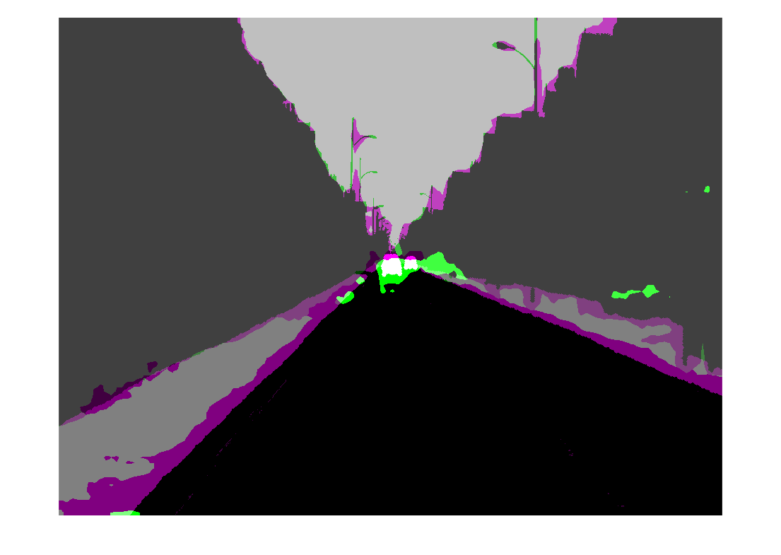
Visually, the semantic segmentation results overlap well for the road, sky, and building classes. However, the results do not overlap well for the car and pavement classes.
Supporting Functions
Model Gradients Function
The helper function modelGradients calculates the gradients and adversarial loss for the generator and discriminator. The function also calculates the segmentation loss for the generator and the cross-entropy loss for the discriminator. As no state information is required to be remembered between the iterations for both generator and discriminator networks, the states are not updated.
function [gradientGenerator, gradientDiscriminator, lossSegValue, lossAdvValue, lossDisValue] = modelGradients(dlnetGenerator, dlnetDiscriminator, dlX, dlZ, label, lamdaAdv)

% Labels for adversarial training.
simulationLabel = 0;
realLabel = 1;

% Extract the predictions of the simulation from the generator.
[genPredictionSimulation, ~] = forward(dlnetGenerator,dlX);

% Compute the generator loss.
lossSegValue = segmentationLoss(genPredictionSimulation,label);

% Extract the predictions of the real data from the generator.
[genPredictionReal, ~] = forward(dlnetGenerator,dlZ);

% Extract the softmax predictions of the real data from the discriminator.
disPredictionReal = forward(dlnetDiscriminator,softmax(genPredictionReal));

% Create a matrix of simulation labels of real prediction size.
Y = simulationLabel * ones(size(disPredictionReal));

% Compute the adversarial loss to make the real distribution close to the simulation label.
lossAdvValue = mse(disPredictionReal,Y)/numel(Y(:));

% Compute the gradients of the generator with regard to loss.
gradientGenerator = dlgradient(lossSegValue + lamdaAdv*lossAdvValue,dlnetGenerator.Learnables);

% Extract the softmax predictions of the simulation from the discriminator.
disPredictionSimulation = forward(dlnetDiscriminator,softmax(genPredictionSimulation));

% Create a matrix of simulation labels of simulation prediction size.
Y = simulationLabel * ones(size(disPredictionSimulation));

% Compute the discriminator loss with regard to simulation class.
lossDisValueSimulation = mse(disPredictionSimulation,Y)/numel(Y(:));

% Extract the softmax predictions of the real data from the discriminator.
disPredictionReal = forward(dlnetDiscriminator,softmax(genPredictionReal));

% Create a matrix of real labels of real prediction size.
Y = realLabel * ones(size(disPredictionReal));

% Compute the discriminator loss with regard to real class.
lossDisValueReal = mse(disPredictionReal,Y)/numel(Y(:));

% Compute the total discriminator loss.
lossDisValue = lossDisValueSimulation + lossDisValueReal;

% Compute the gradients of the discriminator with regard to loss.
gradientDiscriminator = dlgradient(lossDisValue,dlnetDiscriminator.Learnables);

end
Segmentation Loss Function
The helper function segmentationLoss computes the feature segmentation loss, which is defined as the cross-entropy loss for the generator using the simulation data and its respective ground truth. The helper function computes the loss by using the crossentropy function.
function loss = segmentationLoss(predict, target)

% Generate the one-hot encodings of the ground truth.
oneHotTarget = onehotencode(categorical(extractdata(target)),3);

% Convert the one-hot encoded data to dlarray.
oneHotTarget = dlarray(oneHotTarget,'SSCB');

% Compute the softmax output of the predictions.
predictSoftmax = softmax(predict);

% Mask to ignore nans.
mask = ~isnan(oneHotTarget);

% Compute the cross-entropy loss.
loss =  crossentropy(predictSoftmax,oneHotTarget,'ClassificationMode','single-label','Mask',mask)/(numel(oneHotTarget)/2);
end
The helper function downloadDataset downloads both the simulation and real data sets from the specified URLs to the specified folder locations if they do not exist. The function returns the paths of the simulation, real training data, and real testing data. The function downloads the entire CamVid data set and partition the data into training and test sets using the subsetCamVidDatasetFileNames mat file, attached to the example as a supporting file.
function [simulationImagesFolder, simulationLabelsFolder, realImagesFolder, realLabelsFolder,...
    realTestImagesFolder, realTestLabelsFolder] = ...
    downloadDataset(simulationDataLocation, simulationDataURL, realDataLocation, realImageDataURL, realLabelDataURL)

% Build the training image and label folder location for simulation data.
simulationDataZip = fullfile(simulationDataLocation,'SimulationDrivingDataset.zip');

% Get the simulation data if it does not exist.
if ~exist(simulationDataZip,'file')
    mkdir(simulationDataLocation)

    disp('Downloading the simulation data');
    websave(simulationDataZip,simulationDataURL);
    unzip(simulationDataZip,simulationDataLocation);
end

simulationImagesFolder = fullfile(simulationDataLocation,'SimulationDrivingDataset','images');
simulationLabelsFolder = fullfile(simulationDataLocation,'SimulationDrivingDataset','labels');

camVidLabelsZip = fullfile(realDataLocation,'CamVidLabels.zip');
camVidImagesZip = fullfile(realDataLocation,'CamVidImages.zip');

if ~exist(camVidLabelsZip,'file') || ~exist(camVidImagesZip,'file')
    mkdir(realDataLocation)

    disp('Downloading 16 MB CamVid dataset labels...');
    websave(camVidLabelsZip, realLabelDataURL);
    unzip(camVidLabelsZip, fullfile(realDataLocation,'CamVidLabels'));

    disp('Downloading 587 MB CamVid dataset images...');
    websave(camVidImagesZip, realImageDataURL);
    unzip(camVidImagesZip, fullfile(realDataLocation,'CamVidImages'));
end

% Build the training image and label folder location for real data.
realImagesFolder = fullfile(realDataLocation,'train','images');
realLabelsFolder = fullfile(realDataLocation,'train','labels');

% Build the testing image and label folder location for real data.
realTestImagesFolder = fullfile(realDataLocation,'test','images');
realTestLabelsFolder = fullfile(realDataLocation,'test','labels');

% Partition the data into training and test sets if they do not exist.
if ~exist(realImagesFolder,'file') || ~exist(realLabelsFolder,'file') || ...
        ~exist(realTestImagesFolder,'file') || ~exist(realTestLabelsFolder,'file')


    mkdir(realImagesFolder);
    mkdir(realLabelsFolder);
    mkdir(realTestImagesFolder);
    mkdir(realTestLabelsFolder);

    % Load the mat file that has the names for testing and training.
    partitionNames = load('subsetCamVidDatasetFileNames.mat');

    % Extract the test images names.
    imageTestNames = partitionNames.imageTestNames;

    % Remove the empty cells.
    imageTestNames = imageTestNames(~cellfun('isempty',imageTestNames));

    % Extract the test labels names.
    labelTestNames = partitionNames.labelTestNames;

    % Remove the empty cells.
    labelTestNames = labelTestNames(~cellfun('isempty',labelTestNames));

    % Copy the test images to the respective folder.
    for i = 1:size(imageTestNames,1)
        labelSource = fullfile(realDataLocation,'CamVidLabels',labelTestNames(i));
        imageSource = fullfile(realDataLocation,'CamVidImages','701_StillsRaw_full',imageTestNames(i));
        copyfile(imageSource{1}, realTestImagesFolder);
        copyfile(labelSource{1}, realTestLabelsFolder);
    end

    % Extract the train images names.
    imageTrainNames = partitionNames.imageTrainNames;

    % Remove the empty cells.
    imageTrainNames = imageTrainNames(~cellfun('isempty',imageTrainNames));

    % Extract the train labels names.
    labelTrainNames = partitionNames.labelTrainNames;

    % Remove the empty cells.
    labelTrainNames = labelTrainNames(~cellfun('isempty',labelTrainNames));

    % Copy the train images to the respective folder.
    for i = 1:size(imageTrainNames,1)
        labelSource = fullfile(realDataLocation,'CamVidLabels',labelTrainNames(i));
        imageSource = fullfile(realDataLocation,'CamVidImages','701_StillsRaw_full',imageTrainNames(i));
        copyfile(imageSource{1},realImagesFolder);
        copyfile(labelSource{1},realLabelsFolder);
    end
end
end
The helper function addASPPToNetwork creates the atrous spatial pyramid pooling (ASPP) layers and adds them to the input dlnetwork. The function returns the dlnetwork with ASPP layers connected to it.
function net  = addASPPToNetwork(net, numClasses)

% Define the ASPP dilation factors.
asppDilationFactors = [6,12];

% Define the ASPP filter sizes.
asppFilterSizes = [3,3];

% Extract the last layer of the dlnetwork.
lastLayerName = net.Layers(end).Name;

% Define the addition layer.
addLayer = additionLayer(numel(asppDilationFactors),'Name','additionLayer');

% Add the addition layer to the dlnetwork.
net = addLayers(net,addLayer);

% Create the ASPP layers connected to the addition layer
% and connect the dlnetwork.
for i = 1: numel(asppDilationFactors)
    asppConvName = "asppConv_" + string(i);
    branchFilterSize = asppFilterSizes(i);
    branchDilationFactor = asppDilationFactors(i);
    asspLayer  = convolution2dLayer(branchFilterSize, numClasses,'DilationFactor', branchDilationFactor,...
        'Padding','same','Name',asppConvName,'WeightsInitializer','narrow-normal','BiasInitializer','zeros');
    net = addLayers(net,asspLayer);
    net = connectLayers(net,lastLayerName,asppConvName);
    net = connectLayers(net,asppConvName,strcat(addLayer.Name,'/',addLayer.InputNames{i}));
end
end
The helper function predictSegmentationLabelsOnTestSet calculates the confusion matrix of the predicted and ground truth labels using the segmentationConfusionMatrix (Computer Vision Toolbox) function.
function confusionMatrix =  predictSegmentationLabelsOnTestSet(net, minbatchTestData)

confusionMatrix = {};
i = 1;
while hasdata(minbatchTestData)

    % Use next to retrieve a mini-batch from the datastore.
    [dlX, gtlabels] = next(minbatchTestData);

    % Predict the output of the network.
    [genPrediction, ~] = forward(net,dlX);

    % Get the label, which is the index with maximum value in the channel dimension.
    [~, labels] = max(genPrediction,[],3);

    % Get the confusion matrix of each image.
    confusionMatrix{i}  = segmentationConfusionMatrix(double(gather(extractdata(labels))),double(gather(extractdata(gtlabels))));

    i = i+1;
end

confusionMatrix = confusionMatrix';

end
The helper function piecewiseLearningRate computes the current learning rate based on the iteration number.
function lr = piecewiseLearningRate(i, baseLR, numIterations, power)

fraction = i/numIterations;
factor = (1 - fraction)^power * 1e1;
lr = baseLR * factor;

end
The helper function preprocessData performs a zero center shift by subtracting the number of the image channels by the respective mean.
function data = preprocessData(data)

% Extract respective channels.
rc = data(:,:,1);
gc = data(:,:,2);
bc = data(:,:,3);

% Compute the respective channel means.
r = mean(rc(:));
g = mean(gc(:));
b = mean(bc(:));

% Shift the data by the mean of respective channel.
data = single(data) - single(shiftdim([r g b],-1));
end
References
[1] Tsai, Yi-Hsuan, Wei-Chih Hung, Samuel Schulter, Kihyuk Sohn, Ming-Hsuan Yang, and Manmohan Chandraker. “Learning to Adapt Structured Output Space for Semantic Segmentation.” In 2018 IEEE/CVF Conference on Computer Vision and Pattern Recognition, 7472–81. Salt Lake City, UT: IEEE, 2018. https://doi.org/10.1109/CVPR.2018.00780.
[2] Brostow, Gabriel J., Julien Fauqueur, and Roberto Cipolla. “Semantic Object Classes in Video: A High-Definition Ground Truth Database.” Pattern Recognition Letters 30, no. 2 (January 2009): 88–97. https://doi.org/10.1016/j.patrec.2008.04.005.