Classify Defects on Wafer Maps Using Deep Learning
This example shows how to classify eight types of manufacturing defects on wafer maps using a simple convolutional neural network (CNN).
Wafers are thin disks of semiconducting material, typically silicon, that serve as the foundation for integrated circuits. Each wafer yields several individual circuits (ICs), separated into dies. Automated inspection machines test the performance of ICs on the wafer. The machines produce images, called wafer maps, that indicate which dies perform correctly (pass) and which dies do not meet performance standards (fail).
The spatial pattern of the passing and failing dies on a wafer map can indicate specific issues in the manufacturing process. Deep learning approaches can efficiently classify the defect pattern on a large number of wafers. Therefore, by using deep learning, you can quickly identify manufacturing issues, enabling prompt repair of the manufacturing process and reducing waste.
This example shows how to train a classification network that detects and classifies eight types of manufacturing defect patterns. The example also shows how to evaluate the performance of the network.
Download WM-811K Wafer Defect Map Data
This example uses the WM-811K Wafer Defect Map data set [1] [2]. The data set consists of 811,457 wafer maps images, including 172,950 labeled images. Each image has only three pixel values. The value 0 indicates the background, the value 1 represents correctly behaving dies, and the value 2 represents defective dies. The labeled images have one of nine labels based on the spatial pattern of the defective dies. The size of the data set is 3.5 GB.
Set dataDir as the desired location of the data set. Download the data set using the downloadWaferMapData helper function. This function is attached to the example as a supporting file.
dataDir = fullfile(tempdir,"WaferDefects");
downloadWaferMapData(dataDir)
Preprocess and Augment Data
The data is stored in a MAT file as an array of structures. Load the data set into the workspace.
dataMatFile = fullfile(dataDir,"MIR-WM811K","MATLAB","WM811K.mat");
waferData = load(dataMatFile);
waferData = waferData.data;
Explore the data by displaying the first element of the structure. The waferMap field contains the image data. The failureType field contains the label of the defect.
disp(waferData(1))
          waferMap: [45×48 uint8]
           dieSize: 1683
           lotName: 'lot1'
        waferIndex: 1
    trainTestLabel: 'Training'
       failureType: 'none'
Reformat Data
This example uses only labeled images. Remove the unlabeled images from the structure.
unlabeledImages = zeros(size(waferData),"logical");
for idx = 1:size(unlabeledImages,1)
    unlabeledImages(idx) = isempty(waferData(idx).trainTestLabel);
end
waferData(unlabeledImages) = [];
The dieSize, lotName, and waferIndex fields are not relevant to the classification of the images. The example partitions data into training, validation, and test sets using a different convention than specified by trainTestLabel field. Remove these fields from the structure using the rmfield function.
fieldsToRemove = ["dieSize","lotName","waferIndex","trainTestLabel"];
waferData = rmfield(waferData,fieldsToRemove);
Specify the image classes.
defectClasses = ["Center","Donut","Edge-Loc","Edge-Ring", ...
    "Loc","Near-full","Random","Scratch","none"];
numClasses = numel(defectClasses);
Convert the data from a structure to a table with two variables:
WaferImage– Wafer defect map imagesFailureType– Categorical label for each image
waferData = struct2table(waferData);
waferData.Properties.VariableNames = ["WaferImage","FailureType"];
waferData.FailureType = categorical(waferData.FailureType,defectClasses);
Display a sample image from each input image class using the displaySampleWaferMaps helper function. This function is attached to the example as a supporting file.
displaySampleWaferMaps(waferData)

Balance Data By Oversampling
Display the number of images of each class. The data set is heavily unbalanced, with significantly fewer images of each defect class than the number of images without defects.
summary(waferData.FailureType)
     Center           4294
     Donut             555
     Edge-Loc         5189
     Edge-Ring        9680
     Loc              3593
     Near-full         149
     Random            866
     Scratch          1193
     none           147431
To improve the class balancing, oversample the defect classes using the oversampleWaferDefectClasses helper function. This function is attached to the example as a supporting file. The helper function appends the data set with five modified copies of each defect image. Each copy has one of these modifications: horizontal reflection, vertical reflection, or rotation by a multiple of 90 degrees.
waferData = oversampleWaferDefectClasses(waferData);
Display the number of images of each class after class balancing.
summary(waferData.FailureType)
     Center          25764
     Donut            3330
     Edge-Loc        31134
     Edge-Ring       58080
     Loc             21558
     Near-full         894
     Random           5196
     Scratch          7158
     none           147431
Partition Data into Training, Validation, and Test Sets
Split the oversampled data set into training, validation, and test sets using the splitlabels (Computer Vision Toolbox) function. Approximately 90% of the data is used for training, 5% is used for validation, and 5% is used for testing.
labelIdx = splitlabels(waferData,[0.9 0.05 0.05],"randomized",TableVariable="FailureType");
trainingData = waferData(labelIdx{1},:);
validationData = waferData(labelIdx{2},:);
testingData = waferData(labelIdx{3},:);
Augment Training Data
Specify a set of random augmentations to apply to the training data using an imageDataAugmenter object. Adding random augmentations to the training images can avoid the network from overfitting to the training data.
aug = imageDataAugmenter(FillValue=0,RandXReflection=true,RandYReflection=true, ...
    RandRotation=[0 360]);
Read the data using an arrayDatastore object.
inputSize = [48 48];
dsTrain = arrayDatastore(trainingData,"OutputType","same");
dsVal = arrayDatastore(validationData,"OutputType","same");
dsTest = arrayDatastore(testingData,"OutputType","same");
Apply resizing, data augmentation, and one hot encoding of the labels to the training set.
dsTrain = transform(dsTrain,@(x) preprocessAndAugmentTrainingData(x,aug,inputSize));

function dataOut = preprocessAndAugmentTrainingData(dataIn,aug,inputSize)
    failureType = onehotencode(dataIn.FailureType,2);
    waferImage = augment(aug,dataIn.WaferImage{1});
    waferImage = imresize(waferImage,inputSize,'bilinear');
    dataOut = {waferImage,failureType};
end
Apply resizing and one hot encoding to the validation and test sets.
dsVal = transform(dsVal,@(x) preprocessValAndTestData(x,inputSize));
dsTest = transform(dsTest,@(x) preprocessValAndTestData(x,inputSize));

function dataOut = preprocessValAndTestData(dataIn,inputSize)
    failureType = onehotencode(dataIn.FailureType,2);
    waferImage = imresize(dataIn.WaferImage{1},inputSize,'bilinear');
    dataOut = {waferImage,failureType};
end
Create Network
Define the convolutional neural network architecture. The range of the image input layer reflects the fact that the wafer maps have only three levels.
layers = [
    imageInputLayer([inputSize 1], ...
        Normalization="rescale-zero-one",Min=0,Max=2);

    convolution2dLayer(3,8,Padding="same")
    batchNormalizationLayer
    reluLayer

    maxPooling2dLayer(2,Stride=2)

    convolution2dLayer(3,16,Padding="same")
    batchNormalizationLayer
    reluLayer

    maxPooling2dLayer(2,Stride=2)

    convolution2dLayer(3,32,Padding="same")
    batchNormalizationLayer
    reluLayer

    maxPooling2dLayer(2,Stride=2)

    convolution2dLayer(3,64,Padding="same")
    batchNormalizationLayer
    reluLayer

    dropoutLayer

    fullyConnectedLayer(numClasses)
    softmaxLayer];
Specify Training Options
Specify the training options for Adam optimization. Train the network for 30 epochs.
options = trainingOptions("adam", ...
    ResetInputNormalization=true, ...
    MaxEpochs=30, ...
    InitialLearnRate=0.001, ...
    L2Regularization=0.001, ...
    MiniBatchSize=128, ...
    Shuffle="every-epoch", ...
    Verbose=false, ...
    Plots="training-progress", ...
    ValidationData=dsVal, ...
    ValidationFrequency=200);
Train Network or Download Pretrained Network
By default, the example loads a pretrained wafer defect classification network. The pretrained network enables you to run the entire example without waiting for training to complete.
Train the neural network using the trainnet function. For classification, use cross-entropy loss. By default, the trainnet function uses a GPU if one is available. Training on a GPU requires a Parallel Computing Toolbox™ license and a supported GPU device. For information on supported devices, see GPU Computing Requirements (Parallel Computing Toolbox). Otherwise, the trainnet function uses the CPU. To specify the execution environment, use the ExecutionEnvironment training option.
doTraining =false; if doTraining trainedNet = trainnet(dsTrain,layers,@crossentropy,options); modelDateTime = string(datetime("now",Format="yyyy-MM-dd-HH-mm-ss")); save(fullfile(dataDir,"trained-WM811K-"+modelDateTime+".zip"),"trainedNet"); else downloadTrainedWaferNet(fullfile(dataDir,"trainedWM811KCNN_v2")); load(fullfile(dataDir,"trainedWM811KCNN_v2","trained-WM811K.mat")); end
Quantify Network Performance on Test Data
Classify each test image.
defectProbabilities = minibatchpredict(trainedNet,dsTest);
defectPredicted = onehotdecode(defectProbabilities,defectClasses,2);
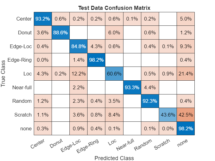
Calculate the performance of the network compared to the ground truth classifications as a confusion matrix using the confusionmat function. Visualize the confusion matrix using the confusionchart function. The values across the diagonal of this matrix indicate correct classifications. The confusion matrix for a perfect classifier has values only on the diagonal.
defectTruth = testingData.FailureType;

cmTest = confusionmat(defectTruth,defectPredicted);
figure
confusionchart(cmTest,categories(defectTruth),Normalization="row-normalized", ...
    Title="Test Data Confusion Matrix");
Precision, Recall, and F1 Scores
This example evaluates the network performance using several metrics: precision, recall, and F1 scores. These metrics are defined for a binary classification. To overcome the limitation for this multiclass problem, you can consider the prediction as a set of binary classifications, one for each class.
Precision is the proportion of images that are correctly predicted to belong to a class. Given the count of true positive (TP) and false positive (FP) classifications, you can calculate precision as:
Recall is the proportion of images belonging to a specific class that were predicted to belong the class. Given the count of TP and false negative (FN) classifications, you can calculate recall as:
F1 scores are the harmonic mean of the precision and recall values:
For each class, calculate the precision, recall, and F1 score using the counts of TP, FP, and FN results available in the confusion matrix.
prTable = table(Size=[numClasses 3],VariableTypes=["cell","cell","double"], ...
    VariableNames=["Recall","Precision","F1"],RowNames=defectClasses);

for idx = 1:numClasses
    numTP = cmTest(idx,idx);
    numFP = sum(cmTest(:,idx)) - numTP;
    numFN = sum(cmTest(idx,:),2) - numTP;

    precision = numTP / (numTP + numFP);
    recall = numTP / (numTP + numFN);

    defectClass = defectClasses(idx);
    prTable.Recall{defectClass} = recall;
    prTable.Precision{defectClass} = precision;
    prTable.F1(defectClass) = 2*precision*recall/(precision + recall);
end
Display the metrics for each class. Scores closer to 1 indicate better network performance.
prTable
prTable=9×3 table
                   Recall      Precision       F1
                 __________    __________    _______

    Center       {[0.9317]}    {[0.9331]}     0.9324
    Donut        {[0.8855]}    {[0.9363]}    0.91022
    Edge-Loc     {[0.8484]}    {[0.8334]}    0.84087
    Edge-Ring    {[0.9817]}    {[0.9648]}     0.9732
    Loc          {[0.6058]}    {[0.9019]}    0.72475
    Near-full    {[0.9333]}    {[0.9767]}    0.95455
    Random       {[0.9231]}    {[0.9125]}    0.91778
    Scratch      {[0.4358]}    {[0.9176]}    0.59091
    none         {[0.9818]}    {[0.9226]}     0.9513
Precision-Recall Curves and Area-Under-Curve (AUC)
In addition to returning a classification of each test image, the network can also predict the probability that a test image is each of the defect classes. In this case, precision-recall curves provide an alternative way to evaluate the network performance.
To calculate precision-recall curves, start by performing a binary classification for each defect class by comparing the probability against an arbitrary threshold. When the probability exceeds the threshold, you can assign the image to the target class. The choice of threshold impacts the number of TP, FP, and FN results and the precision and recall scores. To evaluate the network performance, you must consider the performance at a range of thresholds. Precision-recall curves plot the tradeoff between precision and recall values as you adjust the threshold for the binary classification. The AUC metric summarizes the precision-recall curve for a class as a single number in the range [0, 1], where 1 indicates a perfect classification regardless of threshold.
Use the rocmetrics function to calculate the precision, recall, and AUC for each class over a range of thresholds. Plot the precision-recall curves.
roc = rocmetrics(defectTruth,defectProbabilities,defectClasses, ...
    AdditionalMetrics="prec");
figure
plot(roc,XAxisMetric="reca",YAxisMetric="prec");
xlabel("Recall")
ylabel("Precision")
grid on
title("Precision-Recall Curves for All Classes")
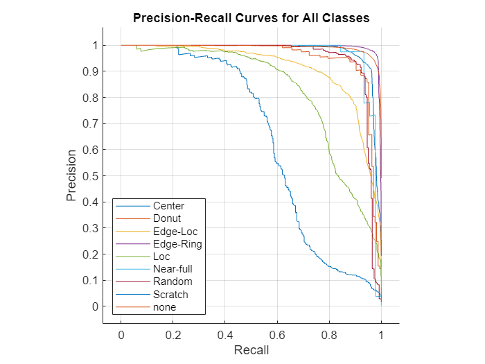
The precision-recall curve for an ideal classifier passes through the point (1, 1). The classes that have precision-recall curves that tend towards (1, 1), such as Edge-Ring and Center, are the classes for which the network has the best performance. The network has the worst performance for the Scratch class.
Compute and display the AUC values of the precision/recall curves for each class.
prAUC = zeros(numClasses, 1);
for idx = 1:numClasses
    defectClass = defectClasses(idx);
    currClassIdx = strcmpi(roc.Metrics.ClassName, defectClass);
    reca = roc.Metrics.TruePositiveRate(currClassIdx);
    prec = roc.Metrics.PositivePredictiveValue(currClassIdx);
    prAUC(idx) = trapz(reca(2:end),prec(2:end)); % prec(1) is always NaN
end
prTable.AUC = prAUC;
prTable
prTable=9×4 table
                   Recall      Precision       F1         AUC
                 __________    __________    _______    _______

    Center       {[0.9317]}    {[0.9331]}     0.9324    0.97642
    Donut        {[0.8855]}    {[0.9363]}    0.91022    0.94845
    Edge-Loc     {[0.8484]}    {[0.8334]}    0.84087    0.91182
    Edge-Ring    {[0.9817]}    {[0.9648]}     0.9732    0.92067
    Loc          {[0.6058]}    {[0.9019]}    0.72475    0.82368
    Near-full    {[0.9333]}    {[0.9767]}    0.95455    0.94337
    Random       {[0.9231]}    {[0.9125]}    0.91778    0.94521
    Scratch      {[0.4358]}    {[0.9176]}    0.59091    0.63495
    none         {[0.9818]}    {[0.9226]}     0.9513    0.99231
Visualize Network Decisions Using Grad-CAM
Gradient-weighted class activation mapping (Grad-CAM) produces a visual explanation of decisions made by the network. You can use the gradCAM function to identify parts of the image that most influenced the network prediction.
Donut Defect Class
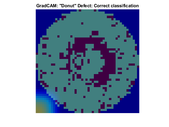
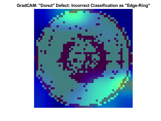
The Donut defect is characterized by an image having defective pixels clustered in a concentric circle around the center of the die. Most images of the Donut defect class do not have defective pixels around the edge of the die.
These two images both show data with the Donut defect. The network correctly classified the image on the left as a Donut defect. The network misclassified the image on the right as an Edge-Ring defect. The images have a color overlay that corresponds to the output of the gradCAM function. The regions of the image that most influenced the network classification appear with bright colors on the overlay. For the image classified as an Edge-Ring defect, the defects at the boundary at the die were treated as important. A possible reason for this could be there are far more Edge-Ring images in the training set as compared to Donut images.
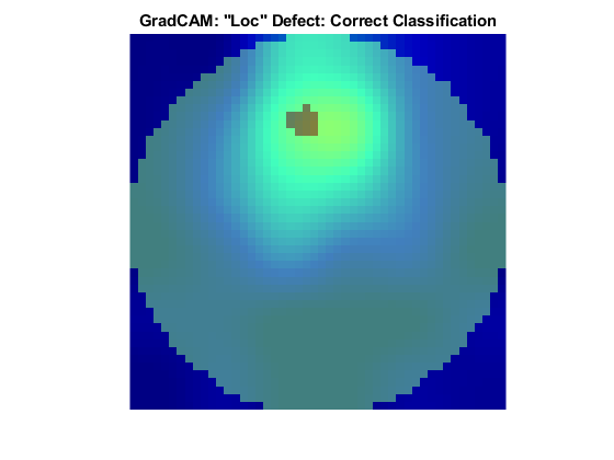
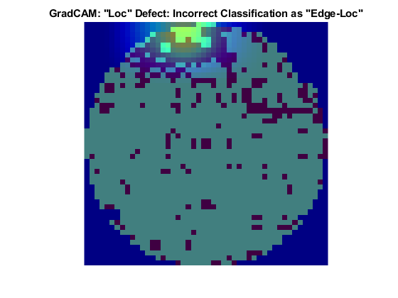
Loc Defect Class
The Loc defect is characterized by an image having defective pixels clustered in a blob away from the edges of the die. These two images both show data with the Loc defect. The network correctly classified the image on the left as a Loc defect. The network misclassified the image on the right and classified the defect as an Edge-Loc defect. For the image classified as an Edge-Loc defect, the defects at the boundary at the die are most influential in the network prediction. The Edge-Loc defect differs from the Loc defect primarily in the location of the cluster of defects.
Compare Correct Classifications and Misclassifications
You can explore other instances of correctly classified and misclassified images. Specify a class to evaluate.
defectClass =  defectClasses(4);
Find the index of all images with the specified defect type as the ground truth or predicted label.
idxTrue = find(testingData.FailureType == defectClass);
idxPred = find(defectPredicted == defectClass);
Find the indices of correctly classified images. Then, select one of the images to evaluate. By default, this example evaluates the first correctly classified image.
idxCorrect = intersect(idxTrue,idxPred);
idxToEvaluateCorrect = 1;
imCorrect = testingData.WaferImage{idxCorrect(idxToEvaluateCorrect)};
1;
imCorrect = testingData.WaferImage{idxCorrect(idxToEvaluateCorrect)};Find the indices of misclassified images. Then, select one of the images to evaluate and get the predicted class of that image. By default, this example evaluates the first misclassified image.
idxIncorrect = setdiff(idxTrue,idxPred);
idxToEvaluateIncorrect = 1;
imIncorrect = testingData.WaferImage{idxIncorrect(idxToEvaluateIncorrect)};
labelIncorrect = defectPredicted(idxIncorrect(idxToEvaluateIncorrect));
1;
imIncorrect = testingData.WaferImage{idxIncorrect(idxToEvaluateIncorrect)};
labelIncorrect = defectPredicted(idxIncorrect(idxToEvaluateIncorrect));Resize the test images to match the input size of the network.
imCorrect = imresize(imCorrect,inputSize);
imIncorrect = imresize(imIncorrect,inputSize);
Generate the score maps using the gradCAM function.
scoreCorrect = gradCAM(trainedNet,imCorrect, ...
testingData.FailureType(idxIncorrect(idxToEvaluateIncorrect)));
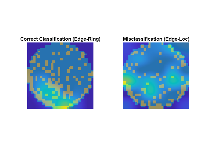
scoreIncorrect = gradCAM(trainedNet,imIncorrect,labelIncorrect);Display the score maps over the original wafer maps using the displayWaferScoreMap helper function. This function is attached to the example as a supporting file.
figure
tiledlayout(1,2)
t = nexttile;
displayWaferScoreMap(imCorrect,scoreCorrect,t)
title("Correct Classification ("+defectClass+")")
t = nexttile;
displayWaferScoreMap(imIncorrect,scoreIncorrect,t)
title("Misclassification ("+string(labelIncorrect)+")")
References
[1] Wu, Ming-Ju, Jyh-Shing R. Jang, and Jui-Long Chen. “Wafer Map Failure Pattern Recognition and Similarity Ranking for Large-Scale Data Sets.” IEEE Transactions on Semiconductor Manufacturing 28, no. 1 (February 2015): 1–12. https://doi.org/10.1109/TSM.2014.2364237.
[2] Jang, Roger. "MIR Corpora." http://mirlab.org/dataset/public/.
[3] Selvaraju, Ramprasaath R., Michael Cogswell, Abhishek Das, Ramakrishna Vedantam, Devi Parikh, and Dhruv Batra. “Grad-CAM: Visual Explanations from Deep Networks via Gradient-Based Localization.” In 2017 IEEE International Conference on Computer Vision (ICCV), 618–26. Venice: IEEE, 2017. https://doi.org/10.1109/ICCV.2017.74.
[4] T., Bex. “Comprehensive Guide on Multiclass Classification Metrics.” October 14, 2021. https://towardsdatascience.com/comprehensive-guide-on-multiclass-classification-metrics-af94cfb83fbd.
See Also
trainnet | trainingOptions | dlnetwork | augmentedImageDatastore | imageDataAugmenter | imageDatastore | minibatchpredict | scores2label | confusionmat | confusionchart
Related Examples
- Detect Image Anomalies Using Explainable FCDD Network
- Detect Image Anomalies Using Pretrained ResNet-18 Feature Embeddings
More About
Select a Web Site
Choose a web site to get translated content where available and see local events and offers. Based on your location, we recommend that you select: United States.
You can also select a web site from the following list
Americas
- América Latina (Español)
- Canada (English)
- United States (English)
Europe
- Belgium (English)
- Denmark (English)
- Deutschland (Deutsch)
- España (Español)
- Finland (English)
- France (Français)
- Ireland (English)
- Italia (Italiano)
- Luxembourg (English)
- Netherlands (English)
- Norway (English)
- Österreich (Deutsch)
- Portugal (English)
- Sweden (English)
- Switzerland
- United Kingdom (English)
Asia Pacific
- Australia (English)
- India (English)
- New Zealand (English)
- 中国
- 日本Japanese (日本語)
- 한국Korean (한국어)