fit
Fit curve or surface to data
Syntax
Description
fitobject = fit(x,y,fitType,fitOptions)fitOptions object.
fitobject = fit(x,y,fitType,Name=Value)fitType with additional options specified by one or more Name=Value pair arguments. Use fitoptions to display available property names and default values for the specific library model.
Examples
Load the census sample data set.
load census;The vectors pop and cdate contain data for the population size and the year the census was taken, respectively.
Fit a quadratic curve to the population data.
f=fit(cdate,pop,'poly2')f =
Linear model Poly2:
f(x) = p1*x^2 + p2*x + p3
Coefficients (with 95% confidence bounds):
p1 = 0.006541 (0.006124, 0.006958)
p2 = -23.51 (-25.09, -21.93)
p3 = 2.113e+04 (1.964e+04, 2.262e+04)
f contains the results of the fit, including coefficient estimates with 95% confidence bounds.
Plot the fit in f together with a scatter plot of the data.
plot(f,cdate,pop)
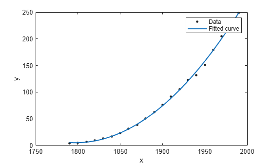
The plot shows that the fitted curve closely follows the population data.
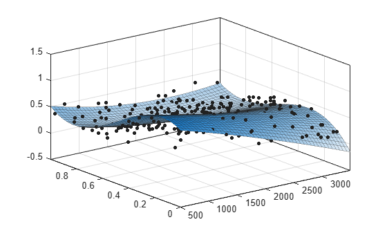
Load the franke sample data set.
load frankeThe vectors x, y, and z contain data generated from Franke's bivariate test function, with added noise and scaling.
Fit a polynomial surface to the data. Specify a degree of two for the x terms and degree of three for the y terms.
sf = fit([x, y],z,'poly23')sf =
Linear model Poly23:
sf(x,y) = p00 + p10*x + p01*y + p20*x^2 + p11*x*y + p02*y^2 + p21*x^2*y
+ p12*x*y^2 + p03*y^3
Coefficients (with 95% confidence bounds):
p00 = 1.118 (0.9149, 1.321)
p10 = -0.0002941 (-0.000502, -8.623e-05)
p01 = 1.533 (0.7032, 2.364)
p20 = -1.966e-08 (-7.084e-08, 3.152e-08)
p11 = 0.0003427 (-0.0001009, 0.0007863)
p02 = -6.951 (-8.421, -5.481)
p21 = 9.563e-08 (6.276e-09, 1.85e-07)
p12 = -0.0004401 (-0.0007082, -0.0001721)
p03 = 4.999 (4.082, 5.917)
sf contains the results of the fit, including coefficient estimates with 95% confidence bounds.
Plot the fit in sf together with a scatterplot of the data.
plot(sf,[x,y],z)
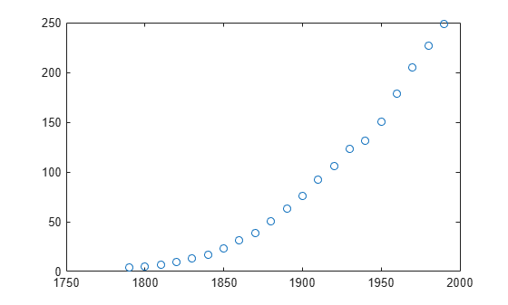
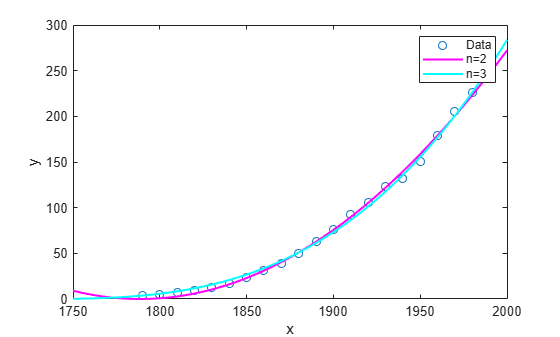
Load and plot the data, create fit options and fit type using the fittype and fitoptions functions, then create and plot the fit.
Load and plot the data in census.mat.
load census
plot(cdate,pop,'o')
Create a fit options object and a fit type for the custom nonlinear model , where a and b are coefficients and n is a problem-dependent parameter.
fo = fitoptions('Method','NonlinearLeastSquares',...
               'Lower',[0,0],...
               'Upper',[Inf,max(cdate)],...
               'StartPoint',[1 1]);
ft = fittype('a*(x-b)^n','problem','n','options',fo);
Fit the data using the fit options and a value of n = 2.
[curve2,gof2] = fit(cdate,pop,ft,'problem',2)curve2 =
General model:
curve2(x) = a*(x-b)^n
Coefficients (with 95% confidence bounds):
a = 0.006092 (0.005743, 0.006441)
b = 1789 (1784, 1793)
Problem parameters:
n = 2
gof2 = struct with fields:
           sse: 246.1543
       rsquare: 0.9980
           dfe: 19
    adjrsquare: 0.9979
          rmse: 3.5994
Fit the data using the fit options and a value of n = 3.
[curve3,gof3] = fit(cdate,pop,ft,'problem',3)curve3 =
General model:
curve3(x) = a*(x-b)^n
Coefficients (with 95% confidence bounds):
a = 1.359e-05 (1.245e-05, 1.474e-05)
b = 1725 (1718, 1731)
Problem parameters:
n = 3
gof3 = struct with fields:
           sse: 232.0058
       rsquare: 0.9981
           dfe: 19
    adjrsquare: 0.9980
          rmse: 3.4944
Plot the fit results with the data.
hold on
plot(curve2,'m')
plot(curve3,'c')
legend('Data','n=2','n=3')
hold off
Load the carbon12alpha nuclear reaction sample data set.
load carbon12alphaangle is a vector of emission angles in radians. counts is a vector of raw alpha particle counts that correspond to the angles in angle.
Display a scatter plot of the counts plotted against the angles.
scatter(angle,counts)
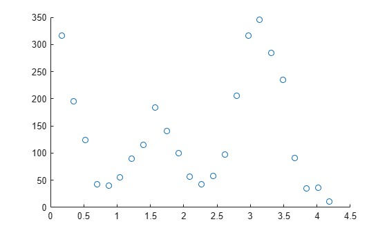
The scatter plot shows that the counts oscillate as the angle increases between 0 and 4.5. To fit a polynomial model to the data, specify the fitType input argument as "poly#" where # is an integer from one to nine. You can fit models of up to nine degrees. See List of Library Models for Curve and Surface Fitting for more information.
Fit a fifth-degree, seventh-degree, and ninth-degree polynomial to the nuclear reaction data. Return the goodness-of-fit statistics for each fit.
[f5,gof5] = fit(angle,counts,"poly5");
[f7,gof7] = fit(angle,counts,"poly7");
[f9,gof9] = fit(angle,counts,"poly9");
Generate a vector of query points between 0 and 4.5 by using the linspace function. Evaluate the polynomial fits at the query points, and then plot them together with the nuclear reaction data.
xq = linspace(0,4.5,1000);

figure
hold on
scatter(angle,counts,"k")
plot(xq,f5(xq))
plot(xq,f7(xq))
plot(xq,f9(xq))
ylim([-100,550])
legend("original data","fifth-degree polynomial","seventh-degree polynomial","ninth-degree polynomial")
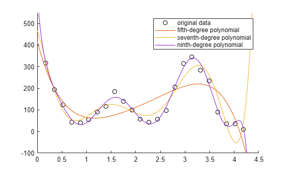
The plot indicates that the ninth-degree polynomial follows the data most closely.
Display the goodness-of-fit statistics for each fit by using the struct2table function.
gof = struct2table([gof5 gof7 gof9],RowNames=["f5" "f7" "f9"])
gof=3×5 table
             sse        rsquare    dfe    adjrsquare     rmse
          __________    _______    ___    __________    ______

    f5    1.0901e+05    0.54614    18      0.42007       77.82
    f7         32695    0.86387    16      0.80431      45.204
    f9        3660.2    0.98476    14      0.97496      16.169
The sum-of-squares error (SSE) for the ninth-degree polynomial fit is smaller than the SSEs for the fifth-degree and seventh-degree fits. This result confirms that the ninth-degree polynomial follows the data most closely.
Load the census sample data set. Fit a cubic polynomial and specify the Normalize (center and scale) and Robust fitting options.
load census;
f = fit(cdate,pop,'poly3','Normalize','on','Robust','Bisquare')
f =
     Linear model Poly3:
     f(x) = p1*x^3 + p2*x^2 + p3*x + p4
       where x is normalized by mean 1890 and std 62.05
     Coefficients (with 95% confidence bounds):
       p1 =     -0.4619  (-1.895, 0.9707)
       p2 =       25.01  (23.79, 26.22)
       p3 =       77.03  (74.37, 79.7)
       p4 =       62.81  (61.26, 64.37)
Plot the fit.
plot(f,cdate,pop)

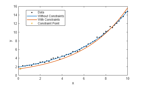
Generate data with an exponential trend and then fit the data using a single-term exponential. Plot the fit and data.
rng(2,"twister");
x = (0:0.2:10)';
y = 2*exp(0.2*x) + 0.2*randn(size(x));

% Without constraints
fitresult1 = fit(x,y,"exp1");
plot(fitresult1,x,y);
hold on

Fit a new exponential curve with the second data point as a constraint. As it is a non-linear fittype, the Algorithm must be specified as "Interior-Point" to fit with constraint points. If it is not specified, the software internally switches to use the "Interior-Point" algorithm.
% With constraints
point = [x(2) y(2)];
fitresult2 = fit(x,y,"exp1",ConstraintPoints=point,Algorithm="Interior-Point");
plot(fitresult2);
plot(point(:,1),point(:,2),"*");
legend("Data","Without Constraints","With Constraints", ...
    "Constraint Point",Location="best");
Define a function in a file and use it to create a fit type and fit a curve.
Define a function in a MATLAB® file.
type piecewiseLine.mfunction y = piecewiseLine(x,a,b,c,k)
% PIECEWISELINE A line made of two pieces
y = zeros(size(x));
% This example includes a for-loop and if statement
% purely for example purposes.
for i = 1:length(x)
if x(i) < k
y(i) = a + b.*x(i);
else
y(i) = a + b*k + c.*(x(i)-k);
end
end
end
Save the file.
Define some data and create a fit type specifying the function piecewiseLine.
x = [0.81;0.91;0.13;0.91;0.63;0.098;0.28;0.55;...
    0.96;0.96;0.16;0.97;0.96];
y = [0.17;0.12;0.16;0.0035;0.37;0.082;0.34;0.56;...
    0.15;-0.046;0.17;-0.091;-0.071];
ft = fittype('piecewiseLine( x, a, b, c, k )')
ft =
     General model:
     ft(a,b,c,k,x) = piecewiseLine( x, a, b, c, k )
The inputs to ft are the coefficients in alphabetical order, followed by the independent variables. See Input Order for Anonymous Functions to learn more.
If you want to control the order of coefficients, then use an anonymous function input. For example, to change the order of the a and b coefficients:
ft = fittype(@(b,a,c,k,x) piecewiseLine(x,a,b,c,k))
You must specify the independent variable x last.
Create a fit using the fit type ft and plot the results.
f = fit(x, y, ft, 'StartPoint', [1, 0, 1, 0.5]);
plot(f, x, y)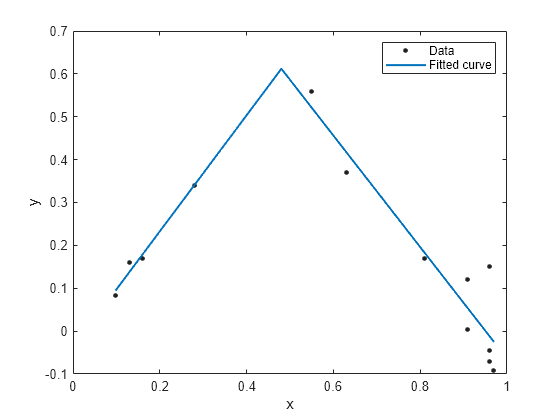
You can define the excluded points as variables before supplying them as inputs to the fit function. The following steps recreate the fits in the previous example and allow you to plot the excluded points as well as the data and the fit.
Load data and define a custom equation and some start points.
[x, y] = titanium;

gaussEqn = 'a*exp(-((x-b)/c)^2)+d'
gaussEqn = 'a*exp(-((x-b)/c)^2)+d'
startPoints = [1.5 900 10 0.6]
startPoints = 1×4

    1.5000  900.0000   10.0000    0.6000
Define two sets of points to exclude, using an index vector and an expression.
exclude1 = [1 10 25];
exclude2 = x < 800;
Create two fits using the custom equation, startpoints, and the two different excluded points.
f1 = fit(x',y',gaussEqn,'Start', startPoints, 'Exclude', exclude1);
f2 = fit(x',y',gaussEqn,'Start', startPoints, 'Exclude', exclude2);
Plot both fits and highlight the excluded data.
plot(f1,x,y,exclude1)
title('Fit with data points 1, 10, and 25 excluded')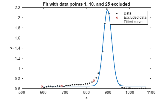
figure;
plot(f2,x,y,exclude2)
title('Fit with data points excluded such that x < 800')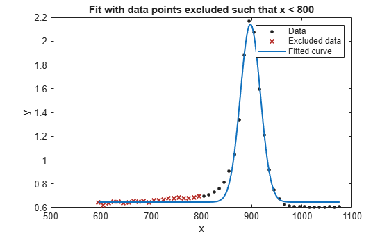
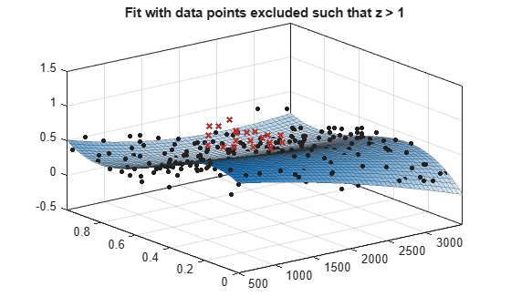
For a surface fitting example with excluded points, load some surface data and create and plot fits specifying excluded data.
load franke
f1 = fit([x y],z,'poly23', 'Exclude', [1 10 25]);
f2 = fit([x y],z,'poly23', 'Exclude', z > 1);

figure
plot(f1, [x y], z, 'Exclude', [1 10 25]);
title('Fit with data points 1, 10, and 25 excluded')
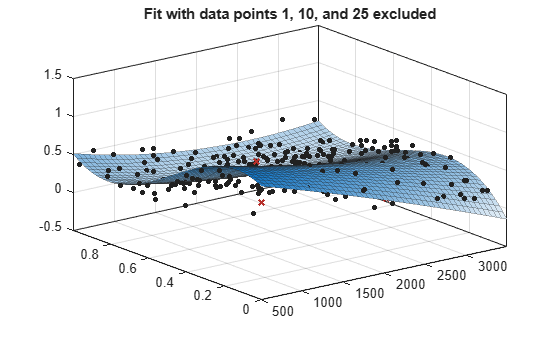
figure
plot(f2, [x y], z, 'Exclude', z > 1);
title('Fit with data points excluded such that z > 1')
Generate some noisy data using the membrane and randn functions.
n = 41;
M = membrane(1,20)+0.02*randn(n);
[X,Y] = meshgrid(1:n);
The matrix M contains data for the L-shaped membrane with added noise. The matrices X and Y contain the row and column index values, respectively, for the corresponding elements in M.
Display a surface plot of the data.
figure(1)
surf(X,Y,M)

The plot shows a wrinkled L-shaped membrane. The wrinkles in the membrane are caused by the noise in the data.
Fit two surfaces through the wrinkled membrane using linear interpolation. For the first surface, specify the linear extrapolation method. For the second surface, specify the extrapolation method as nearest neighbor.
flinextrap = fit([X(:),Y(:)],M(:),"linearinterp",ExtrapolationMethod="linear");
fnearextrap = fit([X(:),Y(:)],M(:),"linearinterp",ExtrapolationMethod="nearest");
Investigate the differences between the extrapolation methods by using the meshgrid function to evaluate the fits at query points extending outside the convex hull of the X and Y data.
[Xq,Yq] = meshgrid(-10:50);

Zlin = flinextrap(Xq,Yq);
Znear = fnearextrap(Xq,Yq);
Plot the evaluated fits.
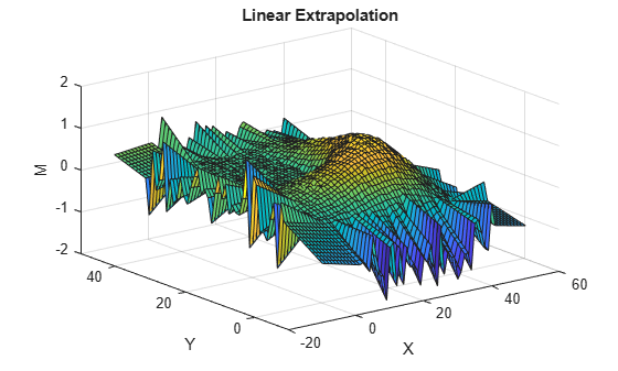
figure(2)
surf(Xq,Yq,Zlin)
title("Linear Extrapolation")
xlabel("X")
ylabel("Y")
zlabel("M")
figure(3)
surf(Xq,Yq,Znear)
title("Nearest Neighbor Extrapolation")
xlabel("X")
ylabel("Y")
zlabel("M")
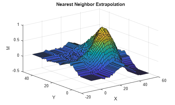
The linear extrapolation method generates spikes outside of the convex hull. The plane segments that form the spikes follow the gradient at points on the convex hull's border. The nearest neighbor extrapolation method uses the data on the border to extend the surface in each direction. This method of extrapolation generates waves that mimic the border.
Fit a smoothing spline curve, and return goodness-of-fit statistics and information about the fitting algorithm.
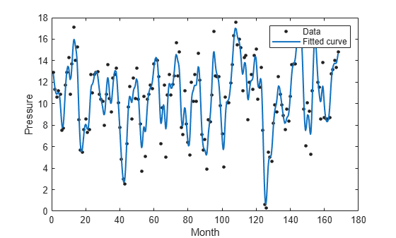
Load the enso sample data set. The enso sample data set contains data for the monthly averaged atmospheric pressure differences between Easter Island and Darwin, Australia.
load enso;Fit a smoothing spline curve to the data in month and pressure, and return goodness-of-fit statistics and the output structure.
[curve,gof,output] = fit(month,pressure,"smoothingspline");Plot the fitted curve with the data used to fit the curve.
plot(curve,month,pressure);
xlabel("Month");
ylabel("Pressure");
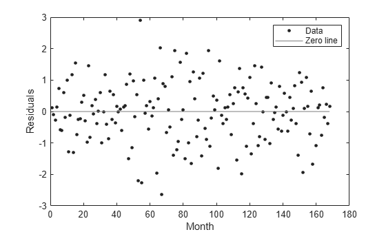
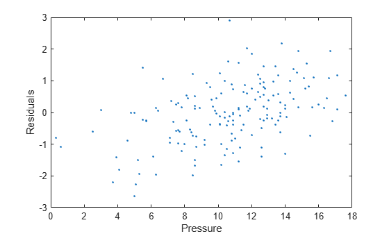
Plot the residuals against the x-data (month).
plot(curve,month,pressure,"residuals")
xlabel("Month")
ylabel("Residuals")
Use the residuals data in the output structure to plot the residuals against the y-data (pressure). To access the residuals field of output, use dot notation.
residuals = output.residuals;
plot( pressure,residuals,".")
xlabel("Pressure")
ylabel("Residuals")
You can use anonymous functions to make it easier to pass other data into the fit function.
Load data and set Emax to 1 before defining your anonymous function:
data = importdata( 'OpioidHypnoticSynergy.txt' );
Propofol      = data.data(:,1);
Remifentanil  = data.data(:,2);
Algometry     = data.data(:,3);
Emax = 1;
Define the model equation as an anonymous function:
Effect = @(IC50A, IC50B, alpha, n, x, y) ...
    Emax*( x/IC50A + y/IC50B + alpha*( x/IC50A )...
    .* ( y/IC50B ) ).^n ./(( x/IC50A + y/IC50B + ...
    alpha*( x/IC50A ) .* ( y/IC50B ) ).^n  + 1);
Use the anonymous function Effect as an input to the fit function, and plot the results:
AlgometryEffect = fit( [Propofol, Remifentanil], Algometry, Effect, ...
    'StartPoint', [2, 10, 1, 0.8], ...
    'Lower', [-Inf, -Inf, -5, -Inf], ...
    'Robust', 'LAR' )
plot( AlgometryEffect, [Propofol, Remifentanil], Algometry )
For more examples using anonymous functions and other custom models for fitting, see the fittype function.
For the properties Upper, Lower, and StartPoint, you need to find the order of the entries for coefficients.
Create a fit type.
ft = fittype('b*x^2+c*x+a');Get the coefficient names and order using the coeffnames function.
coeffnames(ft)
ans = 3×1 cell
    {'a'}
    {'b'}
    {'c'}
Note that this is different from the order of the coefficients in the expression used to create ft with fittype.
Load data, create a fit and set the start points.
load enso
fit(month,pressure,ft,'StartPoint',[1,3,5])
ans =
     General model:
     ans(x) = b*x^2+c*x+a
     Coefficients (with 95% confidence bounds):
       a =       10.94  (9.362, 12.52)
       b =   0.0001677  (-7.985e-05, 0.0004153)
       c =     -0.0224  (-0.06559, 0.02079)
This assigns initial values to the coefficients as follows: a = 1, b = 3, c = 5.
Alternatively, you can get the fit options and set start points and lower bounds, then refit using the new options.
options = fitoptions(ft)
options =
  nlsqoptions with properties:

          StartPoint: []
           Algorithm: 'Trust-Region'
       DiffMinChange: 1.0000e-08
       DiffMaxChange: 0.1000
             Display: 'Notify'
         MaxFunEvals: 600
             MaxIter: 400
              TolFun: 1.0000e-06
                TolX: 1.0000e-06
               Lower: []
               Upper: []
    ConstraintPoints: []
              TolCon: 1.0000e-06
              Robust: 'Off'
           Normalize: 'off'
             Exclude: []
             Weights: []
              Method: 'NonlinearLeastSquares'
options.StartPoint = [10 1 3];
options.Lower = [0 -Inf 0];
fit(month,pressure,ft,options)
ans =
     General model:
     ans(x) = b*x^2+c*x+a
     Coefficients (with 95% confidence bounds):
       a =       10.23  (9.448, 11.01)
       b =   4.335e-05  (-1.82e-05, 0.0001049)
       c =   5.523e-12  (fixed at bound)