Design Internal Model Controller for Chemical Reactor Plant

This example shows how to design a compensator in an IMC structure for series chemical reactors, using Control System Designer. Model-based control systems are often used to track setpoints and reject load disturbances in process control applications.

Plant Model

The plant for this example is a chemical reactor system, comprised of two well-mixed tanks.

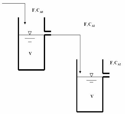
The reactors are isothermal and the reaction in each reactor is first order on component A:

$$r_A=-k{C}_A$$

Material balance is applied to the system to generate a dynamic model of the system. The tank levels are assumed to stay constant because of the overflow nozzle and hence there is no level control involved.

For details about this plant, see Example 3.3 in Chapter 3 of "Process Control: Design Processes and Control Systems for Dynamic Performance" by Thomas E. Marlin.

The following differential equations describe the component balances:

$$V\frac{d{C}_{A1}}{dt}=F(C_{A0}-C_{A1})-Vk{C}_{A1}$$

$$V\frac{d{C}_{A2}}{dt}=F(C_{A1}-C_{A2})-Vk{C}_{A2}$$

At steady state,

$$\frac{d{C}_{A1}}{dt}=0$$

$$\frac{d{C}_{A2}}{dt}=0$$

the material balances are:

$$F^{*}(C_{A0}^{*}-C_{A1}^{*})-Vk{C}_{A1}^{*}=0$$

$$F^{*}(C_{A1}^{*}-C_{A2}^{*})-Vk{C}_{A2}^{*}=0$$

where $$C_{A0}^{*}$$, $$C_{A1}*$$, and $$C_{A2}*$$ are steady-state values.

Substitute the following design specifications and reactor parameters:

• $$F^{*}$$ = 0.085 $$mole/min$$

• $$C_{A0}^{*}$$ = 0.925 $$mol/min$$

• $$V$$ = 1.05 $$m^3$$

• $$k$$ = 0.04 $$mi{n}^{-1}$$

The resulting steady-state concentrations in the two reactors are:

$$C_{A1}^{*}=K{C}_{A0}^{*}=0.6191mol/m^3$$

$$C_{A2}^{*}=K^2{C}_{A0}^{*}=0.4144mol/m^3$$

where

$$K=\frac{F^{*}}{F*+Vk}=0.6693$$

For this example, design a controller to maintain the outlet concentration of reactant from the second reactor, $$C_{A2}^{*}$$, in the presence of any disturbance in feed concentration, $$C_{A0}$$. The manipulated variable is the molar flowrate of the reactant, F, entering the first reactor.

Linear Plant Models

In this control design problem, the plant model is

$$\frac{C_{A2}(s)}{F(s)}$$

and the disturbance model is

$$\frac{C_{A0}(s)}{C_{A2}(s)}$$

This chemical process can be represented using the following block diagram:

where

$$G_{A1}=\frac{C_{A1}(s)}{C_{A0}(s)}=\frac{0.6693}{8.2677s+1}$$

$$G_{F1}=\frac{C_{A1}(s)}{F(s)}=\frac{2.4087}{8.2677s+1}$$

$$G_{A2}=\frac{C_{A2}(s)}{C_{A1}(s)}=\frac{0.6693}{8.2677s+1}$$

$$G_{F2}=\frac{C_{A2}(s)}{F(s)}=\frac{1.6118}{8.2677s+1}$$

Based on the block diagram, obtain the plant and disturbance models as follows:

$$\frac{C_{A2}(s)}{F(s)}=G_{F1}{G}_{A2}+G_{F2}=\frac{13.3259s+3.2239}{(8.2677s+1{)}^2}$$

$$\frac{C_{A2}}{C_{A0}}=G_{A1}{G}_{A2}=\frac{0.4480}{(8.2677s+1{)}^2}$$

Create the plant model at the command line:

s = tf('s');
G1 = (13.3259*s+3.2239)/(8.2677*s+1)^2;
G2 = G1;
Gd = 0.4480/(8.2677*s+1)^2;

G1 is the real plant used in controller evaluation. G2 is an approximation of the real plant and it is used as the predictive model in the IMC structure. G2 = G1 means that there is no model mismatch. Gd is the disturbance model.

Define IMC Structure in Control System Designer

Open Control System Designer. To do so, in the MATLAB desktop, in the Apps tab, select Control System Designer. Alternatively, enter controlSystemDesigner at the MATLAB command prompt.

Select the IMC control architecture. In Control System Designer, click Edit Architecture. In the Edit Architecture dialog box, select Configuration 5.

Load the system data. For G1, G2, and Gd, specify a model Value.

Click OK.

Tune Compensator

When you specify the plant and disturbance models in the Edit Architecture dialog box, Control System Designer updates the displayed plots to reflect your models. The plot on the bottom right shows the closed-loop step response of the system.

Right-click the plot and select Characteristics > Rise Time submenu. Hover your mouse over the rise time marker.

The rise time is about 25 seconds and you want to tune the IMC compensator to achieve a faster closed-loop response time.

To tune the IMC compensator, in Control System Designer, click Tuning Methods, and select Internal Model Control (IMC) Tuning.

Select a Dominant closed-loop time constant of 2 and a Desired controller order of 2.

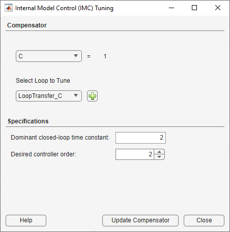
To update the controller, click Update Compensator.

In the closed-loop step response plot, the tuned controller produces a closed-loop rise time around 4.4 seconds.

Control Performance with Model Mismatch

When designing the controller, you assumed G1 was equal to G2. In practice, they are often different, and the controller needs to be robust enough to track setpoints and reject disturbances.

Create model mismatches between G1 and G2 and examine the control performance at the MATLAB® command line in the presence of both setpoint change and load disturbance.

Export the IMC controller to the MATLAB workspace. Click Export. In the Export Model dialog box, select compensator model C.

Click Export.

The app exports the following controller.

C = zpk([-0.121 -0.121],[-0.2419, -0.5],2.5647)

C =
 
  2.5647 (s+0.121)^2
  ------------------
  (s+0.2419) (s+0.5)
 
Continuous-time zero/pole/gain model.

Convert the IMC structure to a classic feedback control structure with the controller in the feedforward path and unit feedback.

C_new = feedback(C,G2,+1)

C_new =
 
               2.5647 (s+0.121)^4
  --------------------------------------------
  (s-0.0004396) (s+0.121) (s+0.1213) (s+0.242)
 
Continuous-time zero/pole/gain model.

Define the following plant models:

• No Model Mismatch:

G1p = (13.3259*s+3.2239)/(8.2677*s+1)^2;

• G1 time constant changed by 5%:

G1t = (13.3259*s+3.2239)/(8.7*s+1)^2;

• G1 gain increased by 3 times:

G1g = 3*(13.3259*s+3.2239)/(8.2677*s+1)^2;

Evaluate the setpoint tracking performance.

step(feedback(G1p*C_new,1),feedback(G1t*C_new,1),feedback(G1g*C_new,1))
legend('No  Mismatch','Mismatch in Time Constant','Mismatch in Gain')

Evaluate the disturbance rejection performance.

step(Gd*feedback(1,G1p*C_new),Gd*feedback(1,G1t*C_new),Gd*feedback(1,G1g*C_new))
legend('No Model Mismatch','Mismatch in Time Constant','Mismatch in Gain')

The controller is fairly robust to uncertainties in the plant parameters.