Main Content

freqsep

Slow-fast decomposition

Description

example

[G1,G2] = freqsep(G,fcut) decomposes a linear dynamic system into slow and fast components around the specified cutoff frequency. The decomposition is G = G1 + G2, where G1 contains all modes with natural frequency less than fcut.

[G1,G2] = freqsep(G,[fmin,fmax]) computes the decomposition where G1 contains all modes with natural frequency fminωnfmax and G2 contains the remaining modes. (since R2023b)

example

[G1,G2] = freqsep(G,___,SepTol=st) sets the accuracy loss factor equal to st. (since R2023b)

[G1,G2,info] = freqsep(___) returns a structure info containing the block-diagonalizing transformation matrices. (since R2023b)

Examples

collapse all

Load a dynamic system model.

load numdemo Pd
bode(Pd)

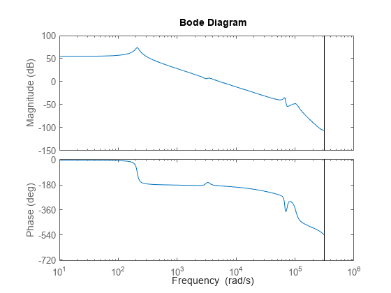
Pd has four complex poles and one real pole. The Bode plot shows a resonance around 210 rad/s and a higher-frequency resonance below 10,000 rad/s.

Decompose this model around 1000 rad/s to separate these two resonances.

[Gs,Gf] = freqsep(Pd,10^3);
bode(Pd,Gs,Gf)
legend('original','slow','fast','Location','Southwest')

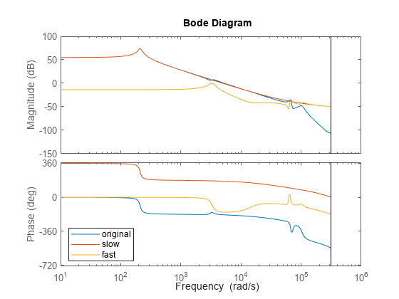
The Bode plot shows that the slow component, Gs, contains only the lower-frequency resonance. This component also matches the DC gain of the original model. The fast component, Gf, contains the higher-frequency resonances and matches the response of the original model at high frequencies. The sum of the two components Gs+Gf yields the original model.

Decompose a model into slow and fast components between poles that are closely spaced.

The following system includes a real pole and a complex pair of poles that are all close to s = -2.

G = zpk(-.5,[-1.9999 -2+1e-4i -2-1e-4i],10);

Try to decompose the model about 2 rad/s, so that the slow component contains the real pole and the fast component contains the complex pair.

[Gs,Gf] = freqsep(G,2);
Warning: One or more fast modes could not be separated from the slow modes. To force separation, relax the accuracy constraint by increasing the "SepTol" factor (see "freqsepOptions" for details).

These poles are too close together for freqsep to separate. Increase the relative tolerance to allow the separation.

[Gs,Gf] = freqsep(G,2,SepTol=5e10);

Now freqsep successfully separates the dynamics.

slowpole = pole(Gs)
slowpole = -1.9999
fastpole = pole(Gf)
fastpole = 2×1 complex

  -2.0000 + 0.0001i
  -2.0000 - 0.0001i

This example shows how to decompose a model and retain the modes in a specified frequency range using freqsep.

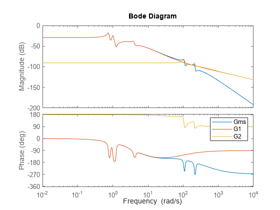
Load the model Gms and examine its frequency response.

load modeselect Gms
bodeplot(Gms)

Use freqsep to retain the dynamics in the frequency range 0.1 rad/s to 50 rad/s.

[G1,G2] = freqsep(Gms,[0.1,50]);

In this decomposition, the output G1 contains all poles with natural frequency in the range [0.1,50] and G2 contains the remaining poles.

bodeplot(Gms,G1,G2)
legend

Input Arguments

collapse all

Dynamic system to decompose, specified as a numeric LTI model, such as a ss or tf model.

Cutoff frequency for fast-slow decomposition, specified as a positive scalar. The output G1 contains all poles with natural frequency less than fcut. The output G2 contains all poles with natural frequency greater than or equal to fcut.

Since R2023b

Frequency range for decomposition, specified as a two-element vector. The output G1 contains all poles with natural frequency in the range [fmin,fmax]. The output G2 contains the remaining poles.

Since R2023b

Accuracy loss factor for slow-fast decomposition, specified as a nonnegative scalar value. freqresp ensures that the frequency responses of the original system, G, and the sum of the decomposed systems G1+G2, differ by no more than SepTol times the absolute accuracy of the computed value of G(s). Increasing SepTol helps separate modes straddling the slow/fast boundary at the expense of accuracy.

Output Arguments

collapse all

Slow dynamics of the decomposed system, returned as a numeric LTI model of the same type as G. G1 contains all poles of G with natural frequency less than fcut, and is such that G = G1 + G2.

Fast dynamics of the decomposed system, returned as a numeric LTI model of the same type as G. Gf contains all poles of G with natural frequency greater than or equal to fcut, and is such that G = G1 + G2.

Since R2023b

Additional information about the decomposition, returned as structure with these fields.

FieldDescription
TLLeft-side matrix of the block-diagonalizing transformation, returned as a matrix with dimensions Nx-by-Nx, where Nx is the number of states in the model G.
TRRight-side matrix of the block-diagonalizing transformation, returned as a matrix with dimensions Nx-by-Nx, where Nx is the number of states in the model G.

The algorithm transforms the state-space realization (A, B, C, D) of the model G to

TLATR=(A100A2),TLB=(B1B2),CTR=(C1C2)

The function returns an empty value [] for this argument when the input model G is not a state-space model.

Alternative Functionality

Live Editor Task

Reduce Model Order

Version History

Introduced in R2014a

expand all