Train PyTorch Channel Prediction Models
This example shows how to train a PyTorch™ based channel prediction neural network using data that you generate in MATLAB.
While this example demonstrates the use of PyTorch for training a channel prediction neural network, the Deep Learning Toolbox provides robust tools for implementing similar models directly within MATLAB.
Introduction
Wireless channel prediction is a crucial aspect of modern communication systems, enabling more efficient and reliable data transmission. Recent advancements in machine learning, particularly neural networks, have introduced a data-driven approach to wireless channel prediction. This approach does not rely on predefined models but instead learns directly from historical channel data. As a result, neural networks can adapt to realistic data, making them less sensitive to disturbances and interference.
Channel prediction using neural networks is fundamentally a time series learning problem since it involves forecasting future channel states based on past estimations. This method is particularly advantageous in environments where spatial correlation is minimal or absent, such as crowded urban areas with numerous moving objects. By focusing on temporal correlations and historical data, neural networks provide a computationally efficient and scalable solution across various environments.
Unlike single‑tap or isotropic scattering models, CDL channels exhibit clustered multipath dynamics and non‑isotropic Doppler spectra, leading to temporal correlations that vary across delay clusters. This motivates the use of gated recurrent unit (GRU) networks, whose nonlinear gates can selectively emphasize relevant temporal structures that linear predictors (e.g., LMMSE/Wiener filters) cannot exploit [1],[2].
PyTorch Code
In this example, you train a GRU network defined in PyTorch. The nr_channel_predictor.py file contains the neural network definition, training and other functionality for the PyTorch network. First create a Python wrapper for the functionality provided in the nr_channel_predictor.py file
The nr_channel_predictor_wrapper.py file contains the interface functions that minimize data transfer between MATLAB and Python processes. This example utilizes the following functions in the nr_channel_predictor_wrapper.py file:
construct_model:Constructs and optionally loads a PyTorch model for channel prediction,train:Trains a channel predictor PyTorch model using offline training,predict:Generates predictions using a trained PyTorch model and input data,save:Saves the state dictionary of a PyTorch model to a file,load:Loads a state dictionary into a PyTorch model from a specified file.
The PyTorch Wrapper Template section shows how to create the interface functions using a template.
The first step of designing an AI-based system is to prepare training and testing data. This example follows the Preprocess Data for AI-Based CSI Feedback Compression example that shows how to preprocess the channel estimates.
Load the preprocessed channel estimates data. If you have run the previous step, then the example uses the data that you prepared in the previous step. Otherwise, the example prepares the data as shown in the Preprocess Data for AI-Based CSI Feedback Compression example.
Generating about 110k samples of training and validation data requires 10 frames of channel realization and takes about 50 seconds using Parallel Computing Toolbox® and a six core Intel® Xeon® W-2133 CPU @ 3.60GHz.
horizon = 10; % ms maxDoppler = 5; if ~exist("inputData","var") || ~exist("targetData","var") || ~exist("dataOptions","var") || ~exist("channel","var") || ~exist("carrier","var") numFrames =10; useParallel =
false; [inputData,targetData,dataOptions,systemParams,channel,carrier] = prepareData(numFrames,useParallel,horizon,maxDoppler); end
Starting channel realization generation
1 worker(s) running
00:00:09 - 10% Completed
00:00:20 - 20% Completed
00:00:30 - 30% Completed
00:00:45 - 40% Completed
00:00:58 - 50% Completed
00:01:09 - 60% Completed
00:01:21 - 70% Completed
00:01:32 - 80% Completed
00:01:43 - 90% Completed
00:01:56 - 100% Completed
00:01:56 - 100% Completed
Starting CSI data preprocessing
1 worker(s) running
00:00:05 - 20% Completed
00:00:11 - 30% Completed
00:00:16 - 40% Completed
00:00:20 - 50% Completed
00:00:24 - 60% Completed
00:00:29 - 70% Completed
00:00:35 - 80% Completed
00:00:39 - 90% Completed
00:00:43 - 100% Completed
00:00:48 - 110% Completed
00:00:48 - 100% Completed
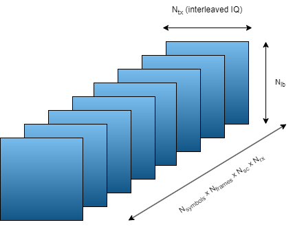
See the channel and carrier variables for current channel and carrier configurations. The inputData variable contains samples of 2-by- arrays, where is the number of transmit antennas and is the number of consecutive slot-spaced time samples.
[Ntxiq,Nseq,Nsamples] = size(inputData)
Ntxiq =
16
Nseq =
68
Nsamples =
124800
Permute the data to bring batches to the first dimension as the PyTorch networks expect batch to be the first dimension.
inputDataPerm = permute(inputData,[3,2,1]);
targetDataPerm = permute(targetData,[2,1]);
Separate the data into training and validation. Define the number of training and validation samples.
numTraining = 90000;
numValidation = 10000;
Randomly sample the input and target data on the time dimension to select training and validation samples. Since each -by- sample is independent, this case has no time continuity requirement.
idxRand = randperm(size(targetDataPerm,1));
Select training and validation data.
xTraining = inputDataPerm(idxRand(1:numTraining),:,:);
xValidation = inputDataPerm(idxRand(1+numTraining:numValidation+numTraining),:,:);
yTraining = targetDataPerm(idxRand(1:numTraining),:);
yValidation = targetDataPerm(idxRand(1+numTraining:numValidation+numTraining),:);
Set Up Python Environment
Before running this example, set up the Python environment as explained in Call Python from MATLAB for Wireless. Specify the full path of the Python executable to use in the pythonPath field below. The helperSetupPyenv function sets the Python environment in MATLAB according to the selected options and checks that the libraries listed in the requirements_chanpre.txt file are installed. This example is tested with Python version 3.11.
if ispc pythonPath =".\.venv\Scripts\pythonw.exe"; else pythonPath =
"./venv_linux/bin/python3"; end requirementsFile = "requirements_chanpre.txt"; executionMode =
"OutOfProcess"; currentPyenv = helperSetupPyenv(pythonPath,executionMode,requirementsFile);
Setting up Python environment
Parsing requirements_chanpre.txt
Checking required package 'numpy'
Checking required package 'torch'
Required Python libraries are installed.
You can use the following process ID and name to attach a debugger to the Python interface and debug the example code.
fprintf("Process ID for '%s' is %s.\n", ...
currentPyenv.ProcessName,currentPyenv.ProcessID)
Process ID for 'MATLABPyHost' is 47596.
Preload the Python module for faster start.
module = py.importlib.import_module('nr_channel_predictor_wrapper');Initiate Neural Network
Initialize the channel predictor neural network. Set GRU hidden size to 128 and number of hidden GRU units to 2. Layer normalization stabilizes training across Doppler conditions, while a dropout rate of 0.3 mitigates overfitting to specific cluster realizations. The chanPredictor variable is the PyTorch model for the GRU based channel predictor.
gruHiddenSize = 128;
gruNumLayers  = 2;
channelInfo = info(channel);
Ntx = channelInfo.NumTransmitAntennas
Ntx =
8
chanPredictor = py.nr_channel_predictor_wrapper.construct_model(...
  Ntx, ...
  gruHiddenSize, ...
  gruNumLayers);

py.nr_channel_predictor_wrapper.info(chanPredictor)
Model architecture:
ChannelPredictorGRU(
  (gru): GRU(16, 128, num_layers=2, batch_first=True, dropout=0.3)
  (layer_norm): LayerNorm((128,), eps=1e-05, elementwise_affine=True)
  (fc): Linear(in_features=128, out_features=16, bias=True)
)

Total number of parameters: 157456
Train Neural Network
The nr_channel_predictor_wrapper.py file contains the MATLAB interface functions to train the channel predictor neural network. Set values for hyperparameters number of epochs, batch size, initial learning rate, validation frequency, and validation patience in epochs. Use early stopping with patience 6 to avoid overfitting, which is especially relevant because CDL realizations contain time‑varying cluster reappearance patterns. Call the train function with required inputs to train and validate the chanPredictor model. Set the verbose variable to true to print out training progress. Training for a maximum epochs of 2000 with early stopping takes more than one hour on a PC that has NVIDIA® TITAN V GPU with a compute capability of 7.0 and 12 GB memory. Set trainNow to true by clicking the check box to train the network. If your GPU runs out of memory during training, reduce the batch size.
trainNow =false; if trainNow numEpochs =
2000; batchSize = 512; initialLearningRate = 3e-3; validationFrequency = 5; validationPatience = 6; verbose = true; tStart = tic; result = py.nr_channel_predictor_wrapper.train( ... chanPredictor, ... xTraining, ... yTraining, ... xValidation, ... yValidation, ... initialLearningRate, ... batchSize, ... numEpochs, ... validationFrequency, ... validationPatience, ... verbose); et = toc(tStart); et = seconds(et); et.Format = "hh:mm:ss.SSS";
The output of the train Python function is a cell array with five elements. The output contains the following in order:
Trained PyTorch model
Training loss array (per iteration)
Validation loss array (per epoch)
Outdated error (with respect to current channel estimate)
Time spent in Python
Parse the function output and display the results.
  chanPredictor = result{1};
  trainingLoss = single(result{2});
  validationLoss = single(result{3});
  elapsedTimePy = result{4};
  bestValidationLoss = result{5}
  bestEpoch = result{6}
  finalEpoch = result{7}
  etInPy = seconds(elapsedTimePy);
  etInPy.Format="hh:mm:ss.SSS";
Save the network for future use together with the training information.
  modelFileName = sprintf("chanpre_gru_hor%d_epochs%d_ts%s",dataOptions.Horizon, ...
    numEpochs,string(datetime("now","Format","dd_MM_HH_mm")));
  fileName = py.nr_channel_predictor_wrapper.save( ...
    chanPredictor, ...
    modelFileName, ...
    Ntx, ...
    gruHiddenSize, ...
    gruNumLayers, ...
    initialLearningRate, ...
    batchSize, ...
    numEpochs, ...
    validationFrequency);
  infoFileName = modelFileName+"_info";
  save(infoFileName,"dataOptions","trainingLoss","validationLoss", ...
    "etInPy","et","initialLearningRate","batchSize","numEpochs","validationFrequency", ...
    "Ntx","gruHiddenSize","gruNumLayers");
  fprintf("Saved network in '%s' file and\nnetwork info in '%s.mat' file.\n", ...
    string(fileName),infoFileName)
else
When called with a filename as the last input, the construct_model function creates a neural network and loads the trained weights from the file. Run the network with xValidation input by calling the predict Python function.
  numEpochs = 2000;
  horizon = 10;
  modelFileName = sprintf("channel_predictor_gru_horizon%d_epochs%d.pth",horizon,numEpochs);
  infoFileName = sprintf("channel_predictor_gru_horizon%d_epochs%d_info.mat",horizon,numEpochs);
  chanPredictor = py.nr_channel_predictor_wrapper.construct_model( ...
    Ntx, ...
    gruHiddenSize, ...
    gruNumLayers, ...
    modelFileName);
  y_out = py.nr_channel_predictor_wrapper.predict( ...
    chanPredictor, ...
    xValidation);
Calculate the mean square error (MSE) loss as compared to the expected channel estimates.
  y = single(y_out);
  bestValidationLoss = mean(sum(abs(y - yValidation).^2,2)/Ntx);
Load the training and validation loss logged during training.
  load(infoFileName,"validationLoss","trainingLoss","etInPy","et")
end
fprintf("Validation Loss: %f dB",10*log10(bestValidationLoss))
Validation Loss: -36.344093 dB
The overhead caused by the Python interface is insignificant.
fprintf("Total training time: %s\nTraining time in Python: %s\nOverhead: %s\n",et,etInPy,et-etInPy)Total training time: 00:16:14.959 Training time in Python: 00:16:13.025 Overhead: 00:00:01.933
Plot the training and validation loss. As the number of iterations increases, the loss value converges to about -37 dB.
figure
plot(10*log10(trainingLoss));
hold on
numIters = size(trainingLoss,2);
iterPerEpoch = numIters/length(validationLoss);
plot(iterPerEpoch:iterPerEpoch:numIters,10*log10(validationLoss),"*-");
hold off
legend("Training", "Validation")
xlabel(sprintf("Iteration (%d iterations per epoch)",iterPerEpoch))
ylabel("Loss (dB)")
title("Training Performance (NMSE as Loss)")
grid on
Investigate Network Performance
Test the network for different horizon values. The helperChanEstCompareNetworks function trains and tests the GRU channel prediction network for the horizon values specified in the horizonVec variable. For robustness, train the GRU with five different random initialization, and pick the model achieving the lowest validation loss.
trainForComparisonNow =false; if trainForComparisonNow horizonVec = [1 2:4:90]; gruHiddenSize = 128; gruNumLayers = 2; numEpochs = 2000; batchSize = 512; initialLearningRate = 3e-3; validationFrequency = 5; validationPatience = 6; if validationFrequency > numEpochs error("numEpocs is less than validationFrequency. Increase " + ... "numEpochs or reduce validationFrequency to collect data.") end compTable = helperChanPreCompareNetworks(channel,carrier, ... dataOptions.InputSequenceLength,horizonVec,gruHiddenSize, ... gruNumLayers,numTraining,numValidation,numEpochs,batchSize, ... initialLearningRate,validationFrequency,validationPatience); save dChannelPredictionNetworkHorizonResults_trials compTable horizonVec numEpochs numTraining numValidation else load dChannelPredictionNetworkHorizonResults compTable horizonVec numEpochs numTraining numValidation end
The plotValidationLoss function plots the simulated validation loss values for all three network architectures. As the prediction horizon increases, the validation loss (NMSE) also increases, reflecting the reduced temporal correlation of the fading process at longer look‑ahead times. In CDL channels, each delay cluster corresponds to a superposition of Doppler components rather than a single Doppler shift, producing multiple characteristic time scales [4]. The nonlinear gating of GRUs can selectively emphasize or suppress these Doppler components depending on the prediction horizon, causing the characteristic rise and oscillations in NMSE beyond ~30 ms, which are not visible in linear minimum mean square error (LMMSE) predictors [3]. Thus, the GRU not only predicts better for short horizons but also reveals physically meaningful temporal structure in CDL fading. Minor non‑monotonic fluctuations in NMSE are expected due to small optimization induced variations during training especially for very low NMSE values.
plotValidationLoss(compTable);
References
[1] W. Jiang and H. D. Schotten, "Recurrent Neural Network-Based Frequency-Domain Channel Prediction for Wideband Communications," 2019 IEEE 89th Vehicular Technology Conference (VTC2019-Spring), Kuala Lumpur, Malaysia, 2019, pp. 1-6, doi: 10.1109/VTCSpring.2019.8746352.
[2] O. Stenhammar, G. Fodor and C. Fischione, "A Comparison of Neural Networks for Wireless Channel Prediction," in IEEE Wireless Communications, vol. 31, no. 3, pp. 235-241, June 2024, doi: 10.1109/MWC.006.2300140.
[3] I. Goodfellow, Y. Bengio, and A. Courville, Deep Learning. Cambridge, MA: MIT Press, 2016.
[4] 3GPP, Study on channel model for frequencies from 0.5 to 100 GHz (Release 19), 3GPP TR 38.901, V19.1.0, Oct. 2025
PyTorch Wrapper Template
You can use your own PyTorch models in MATLAB using the Python interface. The py_wrapper_template.py file provides a simple interface with a predefined API. This example uses the following API set:
construct_model: returns the PyTorch neural network modeltrain: trains the PyTorch modelsave: saves the PyTorch model weights and metadataload: loads the PyTorch model weightsinfo: prints or returns information on the PyTorch model
The Online Training and Testing of PyTorch Model for CSI Feedback Compression example shows an online training workflow and uses the following API set in addition to the one used in this example.
setup_trainer: sets up a trainer object for with online trainingtrain_one_iteration: trains the PyTorch model for one iteration for online trainingvalidate: validates the PyTorch model for online trainingpredict: runs the PyTorch model with the provided input(s)
You can modify the py_wrapper_template.py file. Follow the instruction in the template file to implement the recommended entry points. Delete the entry points that are not relevant to your project. Use the entry point functions as shown in this example to use your own PyTorch models in MATLAB.
Local Functions
function [inputData,targetData,dataOptions,systemParams,channel,carrier,sdsChan] = prepareData(numFrames,useParallel,horizon,maxDoppler) rng(123) carrier = nrCarrierConfig; nSizeGrid = 52; % Number resource blocks (RB) systemParams.SubcarrierSpacing =15; % 15, 30, 60, 120 kHz carrier.NSizeGrid = nSizeGrid; carrier.SubcarrierSpacing = systemParams.SubcarrierSpacing; systemParams.DelayProfile = 'CDL-C'; % 'CDL-A',...,'CDL-E','TDL-A',...,'TDL-E' systemParams.DelaySpread = 300e-9; % s %% Antenna Panel Configuration systemParams.TransmitAntennaArray.NumPanels = 1; % Number of transmit panels in horizontal dimension (Ng) systemParams.TransmitAntennaArray.PanelDimensions = [2 2]; % Number of columns and rows in the transmit panel (N1, N2) systemParams.TransmitAntennaArray.NumPolarizations = 2; % Number of transmit polarizations systemParams.ReceiveAntennaArray.NumPanels = 1; % Number of receive panels in horizontal dimension (Ng) systemParams.ReceiveAntennaArray.PanelDimensions = [2 1]; % Number of columns and rows in the receive panel (N1, N2) systemParams.ReceiveAntennaArray.NumPolarizations = 2; % Number of receive polarizations systemParams.TransmitAntennaArray.NTxAnts = systemParams.TransmitAntennaArray.NumPolarizations*systemParams.TransmitAntennaArray.NumPanels*prod(systemParams.TransmitAntennaArray.PanelDimensions); systemParams.ReceiveAntennaArray.NRxAnts = systemParams.ReceiveAntennaArray.NumPolarizations*systemParams.ReceiveAntennaArray.NumPanels*prod(systemParams.ReceiveAntennaArray.PanelDimensions); systemParams.MaximumDopplerShift = maxDoppler; % Hz systemParams.Carrier = carrier; channel = createChannel(systemParams); Tc = 0.423/systemParams.MaximumDopplerShift; numerology = (systemParams.SubcarrierSpacing/15)-1; Tslot = 1e-3 / 2^numerology; coherenceTimeInSlots = Tc / Tslot; sequenceLength = ceil(coherenceTimeInSlots*0.8); numSlotsPerFrame = sequenceLength + horizon + 10; saveData =
true; dataDir = fullfile(pwd,"Data"); dataFilePrefix = "nr_channel_est"; resetChanel = true; sdsChan = helper3GPPChannelRealizations(... numFrames, ... channel, ... carrier, ... UseParallel=useParallel, ... SaveData=saveData, ... DataDir=dataDir, ... dataFilePrefix=dataFilePrefix, ... NumSlotsPerFrame=numSlotsPerFrame, ... ResetChannelPerFrame=resetChanel); SNR = 20; [sdsPreprocessed,dataOptions] = helperPreprocess3GPPChannelData( ... sdsChan, ... TrainingObjective="prediction", ... AverageOverSlots=false, ... TruncateChannel=false, ... InputSequenceLength=sequenceLength, ... PredictionHorizon=horizon, ... AddNoise=true, ... SNR=SNR, ... DataComplexity="real (interleaved)", ... DataDomain="Frequency-Spatial (FS)", ... UseParallel=useParallel, ... SaveData=saveData); data = readall(sdsPreprocessed); inputCells = cellfun(@(C) C{1}, data, 'UniformOutput', false); targetCells = cellfun(@(C) C{2}, data, 'UniformOutput', false); inputData = cat(3, inputCells{:}); targetData = cat(2, targetCells{:}); featuresMax = max(inputData,[],[2 3]); featuresMin = min(inputData,[],[2 3]); dataMax = max(featuresMax); dataMin = min(featuresMin); inputData = (inputData-dataMin) / (dataMax-dataMin); targetData = (targetData-dataMin) / (dataMax-dataMin); dataOptions.Normalization = "min-max"; dataOptions.MinValue = dataMin; dataOptions.MaxValue = dataMax; dataOptions.Horizon = horizon; end function channel = createChannel(simParameters) % Create and configure the propagation channel. If the number of antennas % is 1, configure only 1 polarization, otherwise configure 2 polarizations. numTxPol = 1 + (simParameters.TransmitAntennaArray.NTxAnts>1); numRxPol = 1 + (simParameters.ReceiveAntennaArray.NRxAnts>1); if contains(simParameters.DelayProfile,'CDL') % Create CDL channel channel = nrCDLChannel; % Tx antenna array configuration in CDL channel. The number of antenna % elements depends on the panel dimensions. The size of the antenna % array is [M,N,P,Mg,Ng]. M and N are the number of rows and columns in % the antenna array. P is the number of polarizations (1 or 2). Mg and % Ng are the number of row and column array panels respectively. Note % that N1 and N2 in the panel dimensions follow a different convention % and denote the number of columns and rows, respectively. txArray = simParameters.TransmitAntennaArray; M = txArray.PanelDimensions(2); N = txArray.PanelDimensions(1); Ng = txArray.NumPanels; channel.TransmitAntennaArray.Size = [M N numTxPol 1 Ng]; channel.TransmitAntennaArray.ElementSpacing = [0.5 0.5 1 1]; % Element spacing in wavelengths channel.TransmitAntennaArray.PolarizationAngles = [-45 45]; % Polarization angles in degrees % Rx antenna array configuration in CDL channel rxArray = simParameters.ReceiveAntennaArray; M = rxArray.PanelDimensions(2); N = rxArray.PanelDimensions(1); Ng = rxArray.NumPanels; channel.ReceiveAntennaArray.Size = [M N numRxPol 1 Ng]; channel.ReceiveAntennaArray.ElementSpacing = [0.5 0.5 1 1]; % Element spacing in wavelengths channel.ReceiveAntennaArray.PolarizationAngles = [0 90]; % Polarization angles in degrees elseif contains(simParameters.DelayProfile,'TDL') channel = nrTDLChannel; channel.NumTransmitAntennas = simParameters.TransmitAntennaArray.NTxAnts; channel.NumReceiveAntennas = simParameters.ReceiveAntennaArray.NRxAnts; else error('Channel not supported.') end % Configure common channel parameters: delay profile, delay spread, and % maximum Doppler shift channel.DelayProfile = simParameters.DelayProfile; channel.DelaySpread = simParameters.DelaySpread; channel.MaximumDopplerShift = simParameters.MaximumDopplerShift; % Configure the channel to return the OFDM response channel.ChannelResponseOutput = 'ofdm-response'; % Get information about the baseband waveform after OFDM modulation step waveInfo = nrOFDMInfo(simParameters.Carrier); % Update channel sample rate based on carrier information channel.SampleRate = waveInfo.SampleRate; end function plotValidationLoss(compTable) horizonVec = compTable.Horizon; metric = "BestValidationLoss"; val = compTable{compTable.Model=="GRU",metric}; if ~isempty(val) plot(horizonVec,10*log10(val),"-*") grid on xlabel("Horizon (ms)") ylabel("Validation Loss") title("GRU Channel Predictor") end end