Preprocess Data for AI-Based CSI Feedback Compression

Since R2025a

This example shows how to preprocess channel estimates and prepare a data set for training an autoencoder for channel state information (CSI) feedback compression. It focuses on the Prepare Data step in the workflow for AI-Based CSI Feedback. You can run each step independently or work through the steps in order.

In this example, you:

1. Preprocess the channel estimates from previously generated data by applying FFT-based transformations to several domains, truncation, normalization, and shaping.

2. Visualize the preprocessed channel estimate.

3. Preprocess a data set of channel estimates in bulk for training neural networks.

For an example of the previous step in the workflow, see Generate MIMO OFDM Channel Realizations for AI-Based Systems.

Channel Realization Data

If the required data is not present in the workspace, this example generates the channel realization data by using the prepareChannelRealizations helper function.

if ~exist("sdsChan","var") || ~exist("channel","var") || ~exist("carrier","var") ...
        || (exist("userParams","var") && ~strcmp(userParams.Preset,"CSI Compression"))
    numSamples = 1000;
[sdsChan,systemParams,channel,carrier] = prepareChannelRealizations(numSamples);
end

Starting parallel pool (parpool) using the 'Processes' profile ...
27-Jan-2026 14:47:04: Job Queued. Waiting for parallel pool job with ID 3 to start ...
Connected to parallel pool with 6 workers.
Starting channel realization generation
6 worker(s) running
00:00:18 - 100% Completed

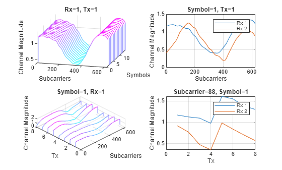
After generating the data, you can view the system configuration by inspecting outputs (stdChan, systemParams, channel, and carrier) of the prepareChannelRealizations helper function.

Preprocess Channel Estimates

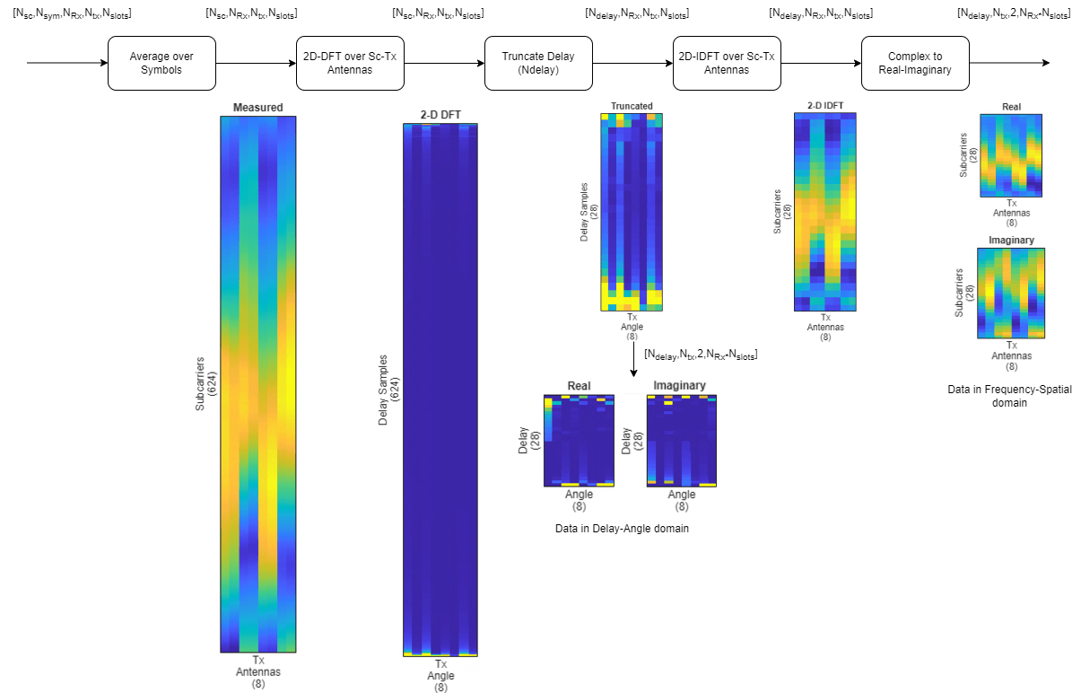
Options to preprocess the channel realizations include applying FFT-based transformations to several domains, truncation, normalization, and shaping. The preprocessing steps are:

• Averaging over slots — If the channel does not change much during a time slot, you can average estimates over the time slots to reduce the noise in the channel estimates and reduce the data size.

• Data domain transformation — The original channel realizations are from subcarriers in the frequency domain and transmit antennas in the spatial domain. Applying FFT-based transformation, you can move the realizations to the delay-angle domain.

• Truncation in delay domain — Most wireless channels present limited delay spread. You can truncate the channel response in the delay domain to reduce the data size. If you apply a final transformation back to the frequency domain, the effect is downsampling in the frequency domain.

• Complex-to-real conversion — To feed complex-valued CSI into standard neural networks, you can map each complex sample into purely real features by expanding the data tensor by one dimension and placing the real (in-phase) and imaginary (quadrature) parts along that new axis.

Preprocessing channel estimates for compression has two possible outputs:

• Delay-angle domain — Real-valued array collected post truncation

• Frequency-spatial domain — Real-valued array collected after 2-D inverse discrete Fourier transform (IDFT)

Assume that the channel coherence time is much larger than the slot time. Average the channel estimate over a slot and obtain a $\left[N_{\text{subcarriers}}1N_{\text{rx}}{N}_{\text{tx}}\right]$ array.

reset(sdsChan)
Hest = read(sdsChan);
[Nsc,~,~,Ntx] = size(Hest);
Hmean = squeeze(mean(Hest,2));

To enable operation on subcarriers and Tx antennas, move the Tx and Rx antenna dimensions to the second and third dimensions, respectively.

Hmean = permute(Hmean,[1 3 2]);

To obtain the delay-angle representation of the channel, apply a 2-D discrete Fourier transform (DFT) over subcarriers and Tx antennas for each Rx antenna and slot.

Hdft2 = fft2(Hmean);

Since the multipath delay in the channel is limited, truncate the delay dimension to remove values that do not carry information. The sampling period on the delay dimension is $T_{\text{delay}}=1/\left(N_{\text{subcarriers}}\ast F_{\text{ss}}\right)$, where $F_{\text{ss}}$ is subcarrier spacing. The expected RMS delay spread in delay samples is ${\tau }_{\text{RMS}}/T_{\text{delay}}$, where ${\tau }_{\text{RMS}}$ is the RMS delay spread of the channel in seconds.

Tdelay = 1/(Nsc*carrier.SubcarrierSpacing*1e3);
rmsTauSamples = channel.DelaySpread/Tdelay;
maxTruncationFactor = floor(Nsc/rmsTauSamples);

Truncate the channel estimate to an even number of samples that is 10 times the expected RMS delay spread. Increasing the TruncationFactor value decreases loss due to preprocessing, but it increases the neural network complexity, the number of required training data points, and the training time. A neural network with more learnable parameters might not converge to a better solution.

dataOptions.TruncationFactor = 10;
dataOptions.MaxDelay = round((channel.DelaySpread/Tdelay)*dataOptions.TruncationFactor/2)*2

dataOptions = struct with fields:
    TruncationFactor: 10
            MaxDelay: 28

Calculate the truncation indices and truncate the channel estimate.

midPoint = floor(Nsc/2);
lowerEdge = midPoint - (Nsc-dataOptions.MaxDelay)/2 + 1;
upperEdge = midPoint + (Nsc-dataOptions.MaxDelay)/2;
Htemp = Hdft2([1:lowerEdge-1 upperEdge+1:end],:,:);

Select the domain for preprocessed data preparation in the delay-angle domain or frequency-spatial domain.

dataOptions.DataDomain = "Frequency-Spatial (FS)";
switch dataOptions.DataDomain
  case "Delay-Angle (DA)"
        Htrunc = Htemp;
        xLabelStr = "Angle";
        yLabelStr = "Delay";
    case "Frequency-Spatial (FS)"
        Htrunc = ifft2(Htemp);
        xLabelStr = "Tx Antennas";
        yLabelStr = "Subcarriers";
end

Separate Real and Imaginary Parts

Since the truncated channel data is complex and the network requires real-valued data, separate the real and imaginary parts. Combine these components on the third dimension to create an $$N_D$$-by-$$N_{tx}$$-by-2-by-$$N_{samples}$$ array, where $$N_{samples}$$ is equal to $$N_{rx}$$ for a single frame.

HtruncReal = permute(cat(4, real(Htrunc), imag(Htrunc)),[1 2 4 3]);
size(HtruncReal)

ans = 1×4

    28    8    2    2

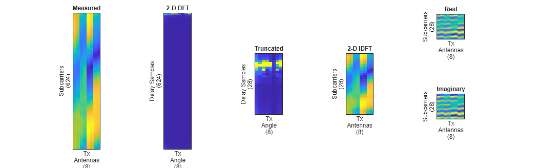
Visualize Channel Estimate Data

Plot the channel estimate signal at each stage of the preprocessing.

helperPlotCSIFeedbackPreprocessingSteps(Hmean(:,:,1), ...
Hdft2(:,:,1), Htemp(:,:,1), ...
Htrunc(:,:,1), Nsc, ...
Ntx, ...
dataOptions.MaxDelay, ...
dataOptions.DataDomain);

Preprocess Data in Bulk

The helperPreprocess3GPPChannelData helper function preprocesses the channel realizations saved in files in the dataDir directory. The helper function takes the sdsChan signal datastore as its first input to load the channel realizations and optionally saves the preprocessed data to the processed folder in the dataDir directory.

Set TrainingObjective to "autocoding" to generate preprocessed channel realizations that you can use as the input signal and the target signal of an autoencoder. Set AverageOverSlots to true. To enable truncation in the delay domain, set TruncateChannel to true and specify the truncation factor and expected delay spread in samples.

[sdsProcessed,dataOptions] = helperPreprocess3GPPChannelData( ...
sdsChan, ...
DataDomain=dataOptions.DataDomain, ...
TrainingObjective="autoencoding", ...
AverageOverSlots=true, ...
TruncateChannel=true, ...
TruncationFactor=dataOptions.TruncationFactor, ...
SaveData=true, ...
UseParallel=true, ...
ExpectedDelaySpreadSamples=rmsTauSamples);

Starting CSI data preprocessing
6 worker(s) running
00:00:07 - 100% Completed

Access the data files using the returned signal datastore. The show the size and dimension of the data samples, display a sample.

sdsProcessed.SignalVariableNames = "inputData";
inputDataCell = readall(sdsProcessed);
size(inputDataCell{1})

ans = 1×4

    28    8    2    2

inputData = cat(4,inputDataCell{:});
[maxDelay,nTx,Niq,Nsamples] = size(inputData)

maxDelay = 
28

nTx = 
8

Niq = 
2

Nsamples = 
2000

figure
subplot(1,2,1)
imagesc(inputData(:,:,1,1,1))
xlabel(xLabelStr)
ylabel(yLabelStr)
title("In-Phase")
subplot(1,2,2)
imagesc(inputData(:,:,2,1,1))
xlabel(xLabelStr)
ylabel(yLabelStr)
title("Quadrature")

Apply Mean-Variance Normalization

Before feeding the channel estimates into the network, apply a two‐step mean-variance normalization with affine rescaling to both the real and imaginary parts:

• Z-score standardization: $$Z=\frac{X-\mu }{\sigma }$$

  • $$X$$ is the raw channel estimate.

  • $$\mu$$ is the sample mean.

  • $$\sigma$$ is the sample standard deviation.

• Affine rescaling: $$X_{\text{norm}}=Z\times {\sigma }_{\text{target}}+0.5$$

  • $${\sigma }_{\text{target}}$$ is the desired standard deviation of the normalized data.

  • Shift by 0.5 to center the values around 0.5.

meanVal = mean(inputData,'all')

meanVal = single

-0.0111

stdVal = std(inputData,[],'all')

stdVal = single

0.7132

inputData = (inputData-meanVal) / stdVal;
targetStd = 0.0212;
inputData = inputData*targetStd+0.5;

This normalization ensures that all network inputs have a consistent scale and distribution, which can improve convergence speed and stability during training. Save the normalization parameters.

dataOptions.MeanValue = meanVal;
dataOptions.StandardDeviationValue = stdVal;
dataOptions.TargetStandardDeviation = targetStd;

Preprocess Data Using Transform Datastore

Alternatively, preprocess the data using a transform datastore, where the transform function is the preconfigured helperPreprocess3GPPChannelData function. Normalize the data using the previously determined the minimum and maximum normalization parameters. The transform function creates a new datastore, tdsChan, that applies preprocessing to the data read from the underlying datastore, sdsChan. This preprocessing method is particularly useful when dealing with large data sets that cannot fit entirely in memory. Because the readall function uses the parallel pool to load data, UseParallel must be set to false when calling helperPreprocess3GPPChannelData.

tdsChan = transform(sdsChan, @(x){helperPreprocess3GPPChannelData( ...
  x, ...
  DataDomain=dataOptions.DataDomain, ...
  TrainingObjective="autoencoding", ...
  AverageOverSlots=true, ...
  TruncateChannel=true, ...
  TruncationFactor=dataOptions.TruncationFactor, ...
  SaveData=false, ...
  UseParallel=false, ...
  Verbose=false, ...
  ExpectedDelaySpreadSamples=rmsTauSamples, ...
  Normalization="mean-variance", ...
  MeanValue=dataOptions.MeanValue, ...
  StandardDeviationValue=dataOptions.StandardDeviationValue, ...
  TargetStandardDeviation=dataOptions.TargetStandardDeviation)});

Read all the data and apply preprocessing.

inputDataCell = readall(tdsChan,UseParallel=true);
inputData2 = cat(4,inputDataCell{:});
[maxDelay,nTx,Niq,Nsamples] = size(inputData2)

maxDelay = 
2

nTx = 
1

Niq = 
1

Nsamples = 
1000

Further Exploration

After preprocessing channel realizations, you can use the CSI snapshots to explore channel feedback compression neural network training in these examples:

• Train Autoencoders for CSI Feedback Compression — Design, train, and evaluate an autoencoder for CSI compression and reconstruction.

• CSI Feedback with Transformer Autoencoder — Design, train, and evaluate a transformer autoencoder for CSI compression and reconstruction.

You can also explore how to use this generated data to train and test neural networks based on PyTorch® and Keras models hosted in MATLAB®:

• Offline Training and Testing of PyTorch Model for CSI Feedback Compression

• Online Training and Testing of PyTorch Model for CSI Feedback Compression

• CSINet Channel Compression in MATLAB Using Keras

For information about the full workflow, see AI-Based CSI Feedback.

Local Functions

function [sdsChan,systemParams,channel,carrier] = prepareChannelRealizations(numSamples)
carrier = nrCarrierConfig;
nSizeGrid = 52;                                         % Number resource blocks (RB)
systemParams.SubcarrierSpacing = 15;  % 15, 30, 60, 120 kHz
carrier.NSizeGrid = nSizeGrid;
carrier.SubcarrierSpacing = systemParams.SubcarrierSpacing;
waveInfo = nrOFDMInfo(carrier);
systemParams.TxAntennaSize = [2 2 2 1 1];   % rows, columns, polarization, panels
systemParams.RxAntennaSize = [2 1 1 1 1];   % rows, columns, polarization, panels
systemParams.MaxDoppler = 5;                % Hz
systemParams.RMSDelaySpread = 300e-9;       % s
systemParams.DelayProfile = "CDL-C"; % CDL-A, CDL-B, CDL-C, CDL-D, CDL-D, CDL-E
channel = nrCDLChannel;
channel.DelayProfile = systemParams.DelayProfile;
channel.DelaySpread = systemParams.RMSDelaySpread;     % s
channel.MaximumDopplerShift = systemParams.MaxDoppler; % Hz
channel.RandomStream = "Global stream";
channel.TransmitAntennaArray.Size = systemParams.TxAntennaSize;
channel.ReceiveAntennaArray.Size = systemParams.RxAntennaSize;
channel.ChannelFiltering = false;
channel.SampleRate = waveInfo.SampleRate;
samplesPerSlot = ...
  sum(waveInfo.SymbolLengths(1:waveInfo.SymbolsPerSlot));
slotsPerFrame = 1;
channel.NumTimeSamples = samplesPerSlot*slotsPerFrame;
systemParams.NumSymbols = slotsPerFrame*14;
useParallel = true;
saveData =  true;
dataDir = fullfile(pwd,"Data");
dataFilePrefix = "nr_channel_est";
numSlotsPerFrame = 1;
resetChanel = true;
sdsChan = helper3GPPChannelRealizations(...
  numSamples, ...
  channel, ...
  carrier, ...
  UseParallel=useParallel, ...
  SaveData=saveData, ...
  DataDir=dataDir, ...
  dataFilePrefix=dataFilePrefix, ...
  NumSlotsPerFrame=numSlotsPerFrame, ...
  ResetChannelPerFrame=resetChanel);
end

function helperPlotCSIFeedbackPreprocessingSteps(Hmean,Hdft2,Htemp,Htrunc, ...
    nSub,nTx,maxDelay,dataDomain)
% helperPlotCSIFeedbackPreprocessingSteps Plot preprocessing workflow

hfig = figure;
hfig.Position(3) = hfig.Position(3)*2;
subplot(2,5,[1 6])
himg = imagesc(abs(Hmean));
himg.Parent.YDir = "normal";
himg.Parent.Position(3) = 0.05;
himg.Parent.XTick=''; himg.Parent.YTick='';
xlabel(sprintf('Tx\nAntennas\n(%d)',nTx));
ylabel(sprintf('Subcarriers\n(%d)',nSub'));
title("Measured")
subplot(2,5,[2 7])
himg = image(abs(Hdft2));
himg.Parent.YDir = "normal";
himg.Parent.Position(3) = 0.05;
himg.Parent.XTick=''; himg.Parent.YTick='';
title("2-D DFT")
xlabel(sprintf('Tx\nAngle\n(%d)',nTx));
ylabel(sprintf('Delay Samples\n(%d)',nSub'));
subplot(2,5,[3 8])
himg = image(abs(Htemp));
himg.Parent.YDir = "normal";
himg.Parent.Position(3) = 0.05;
himg.Parent.Position(4) = himg.Parent.Position(4)*10*maxDelay/nSub;
himg.Parent.Position(2) = (1 - himg.Parent.Position(4)) / 2;
himg.Parent.XTick=''; himg.Parent.YTick='';
xlabel(sprintf('Tx\nAngle\n(%d)',nTx));
ylabel(sprintf('Delay Samples\n(%d)',maxDelay'));
title("Truncated")
if strcmpi(dataDomain,"Frequency-Spatial (FS)")
    subplot(2,5,[4 9])
    himg = imagesc(abs(Htrunc));
    himg.Parent.YDir = "normal";
    himg.Parent.Position(3) = 0.05;
    himg.Parent.Position(4) = himg.Parent.Position(4)*10*maxDelay/nSub;
    himg.Parent.Position(2) = (1 - himg.Parent.Position(4)) / 2;
    himg.Parent.XTick=''; himg.Parent.YTick='';
    xlabel(sprintf('Tx\nAntennas\n(%d)',nTx));
    ylabel(sprintf('Subcarriers\n(%d)',maxDelay'));
    title("2-D IDFT")
    subplot(2,5,5)
    himg = imagesc(real(Htrunc));
    himg.Parent.YDir = "normal";
    himg.Parent.Position(3) = 0.05;
    himg.Parent.Position(4) = himg.Parent.Position(4)*10*maxDelay/nSub;
    himg.Parent.Position(2) = himg.Parent.Position(2) + 0.18;
    himg.Parent.XTick=''; himg.Parent.YTick='';
    xlabel(sprintf('Tx\nAntennas\n(%d)',nTx));
    ylabel(sprintf('Subcarriers\n(%d)',maxDelay'));
    title("Real")
    subplot(2,5,10)
    himg = imagesc(imag(Htrunc));
    himg.Parent.YDir = "normal";
    himg.Parent.Position(3) = 0.05;
    himg.Parent.Position(4) = himg.Parent.Position(4)*10*maxDelay/nSub;
    himg.Parent.Position(2) = himg.Parent.Position(2) + 0.18;
    himg.Parent.XTick=''; himg.Parent.YTick='';
    xlabel(sprintf('Tx\nAntennas\n(%d)',nTx));
    ylabel(sprintf('Subcarriers\n(%d)',maxDelay'));
    title("Imaginary")
elseif strcmpi(dataDomain,"Delay-Angle (DA)")
    subplot(2,5,4)
    himg = image(real(Htrunc));
    himg.Parent.YDir = "normal";
    himg.Parent.Position(3) = 0.05;
    himg.Parent.Position(4) = himg.Parent.Position(4)*10*maxDelay/nSub;
    himg.Parent.Position(2) = himg.Parent.Position(2) + 0.18;
    himg.Parent.XTick=''; himg.Parent.YTick='';
    xlabel(sprintf('Angle\n(%d)',nTx));
    ylabel(sprintf('Delay\n(%d)',maxDelay'));
    title("Real")
    subplot(2,5,9)
    himg = image(imag(Htrunc));
    himg.Parent.YDir = "normal";
    himg.Parent.Position(3) = 0.05;
    himg.Parent.Position(4) = himg.Parent.Position(4)*10*maxDelay/nSub;
    himg.Parent.Position(2) = himg.Parent.Position(2) + 0.18;
    himg.Parent.XTick=''; himg.Parent.YTick='';
    xlabel(sprintf('Angle\n(%d)',nTx));
    ylabel(sprintf('Delay\n(%d)',maxDelay'));
    title("Imaginary")
end
end

References

[1] 3GPP TR 38.901. "Study on channel model for frequencies from 0.5 to 100 GHz." 3rd Generation Partnership Project; Technical Specification Group Radio Access Network.

[2] Wen, Chao-Kai, Wan-Ting Shih, and Shi Jin. "Deep Learning for Massive MIMO CSI Feedback." IEEE Wireless Communications Letters 7, no. 5 (October 2018): 748–51. https://doi.org/10.1109/LWC.2018.2818160.

[3] Zimaglia, Elisa, Daniel G. Riviello, Roberto Garello, and Roberto Fantini. "A Novel Deep Learning Approach to CSI Feedback Reporting for NR 5G Cellular Systems." In 2020 IEEE Microwave Theory and Techniques in Wireless Communications (MTTW), 47–52. Riga, Latvia: IEEE, 2020. https://doi.org/10.1109/MTTW51045.2020.9245055.