Hauptinhalt

plot

Display RF propagation rays in Site Viewer

Description

plot(rays) displays the specified propagation rays in Site Viewer.

example

plot(rays,Name=Value) displays the rays using additional options specified by name-value arguments.

Examples

collapse all

Perform ray tracing in Chicago and return the rays in comm.Ray objects. Then, display the rays without performing the ray tracing analysis again.

Launch Site Viewer with buildings in Chicago. For more information about the OpenStreetMap® file, see [1].

viewer = siteviewer(Buildings="chicago.osm");

Site Viewer with buildings

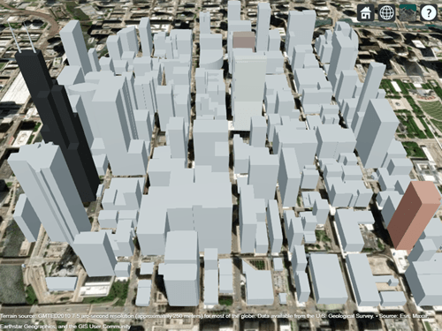
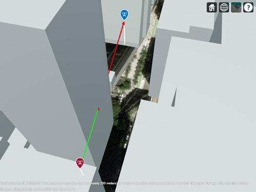
Create a transmitter site on one building and a receiver site on another building. Show the line-of-sight path between the sites using the los function.

tx = txsite(Latitude=41.8800, ...
    Longitude=-87.6295, ...
    TransmitterFrequency=2.5e9);
rx = rxsite(Latitude=41.881352, ...
    Longitude=-87.629771, ...
    AntennaHeight=30);
los(tx,rx)

Obstructed line-of-sight path from the transmitter site to the receiver site. The path is green from the transmitter to the building, and red from the building to the receiver.

Create a ray tracing propagation model, which MATLAB® represents using a RayTracing object. By default, the model uses the SBR method and calculates propagation paths with up to two reflections.

pm = propagationModel("raytracing");

Perform the ray tracing analysis. The raytrace function returns a cell array containing the comm.Ray objects.

rays = raytrace(tx,rx,pm)
rays = 1×1 cell array
    {1×3 comm.Ray}

View the properties of the first ray object.

rays{1}(1)
ans = 
  Ray with properties:

      PathSpecification: 'Locations'
       CoordinateSystem: 'Geographic'
    TransmitterLocation: [3×1 double]
       ReceiverLocation: [3×1 double]
            LineOfSight: 0
           Interactions: [1×1 struct]
              Frequency: 2.5000e+09
         PathLossSource: 'Custom'
               PathLoss: 92.7686
             PhaseShift: 1.2945

   Read-only properties:
       PropagationDelay: 5.7088e-07
    PropagationDistance: 171.1462
       AngleOfDeparture: [2×1 double]
         AngleOfArrival: [2×1 double]
        NumInteractions: 1

Close Site Viewer.

close(viewer)

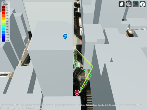
Create another Site Viewer with the same buildings, transmitter site, and receiver site. Then, display the propagation paths. Alternatively, you can plot individual paths by specifying a single ray object, for example rays{1}(2).

siteviewer(Buildings="chicago.osm");
show(tx)
show(rx)
plot(rays{1},Type="power", ...
    TransmitterSite=tx,ReceiverSite=rx)

Three propagation paths from the transmitter site to the receiver site

Appendix

[1] The OpenStreetMap file is downloaded from https://www.openstreetmap.org, which provides access to crowd-sourced map data all over the world. The data is licensed under the Open Data Commons Open Database License (ODbL), https://opendatacommons.org/licenses/odbl/.

Input Arguments

collapse all

Propagation rays, specified as a comm.Ray object or a vector of comm.Ray objects. The PathSpecification property of the ray must be "Locations".

Name-Value Arguments

collapse all

Specify optional pairs of arguments as Name1=Value1,...,NameN=ValueN, where Name is the argument name and Value is the corresponding value. Name-value arguments must appear after other arguments, but the order of the pairs does not matter.

Example: plot(rays,Type="pathloss",ColorLimits=[-100 0]) adjusts the default color limits of the plotted ray.

Before R2021a, use commas to separate each name and value, and enclose Name in quotes.

Example: plot(rays,"Type","pathloss","ColorLimits",[-100 0]) adjusts the default color limits of the plotted ray.

Type of quantity to plot, specified as one of these options:

  • "pathloss" — The color of the path indicates the path loss in dB.

  • "power" — The color of the path indicates the power of the signal in dBm.

Data Types: char | string

Transmitter site, specified as a txsite object.

Dependencies

This name-value argument applies only when Type is set to "power".

Data Types: char

Receiver site, specified as an rxsite object.

Dependencies

This name-value argument applies only when Type is set to "power".

Data Types: char

Color limits for the colormap, specified as a 1-by-2 vector of the form [cmin cmax]. The value of cmin must be less than the value of cmax. cmin represents the lower saturation limit and cmax represents the upper saturation limit.

The default value is [-120 -5] when Type is "power" and [45 160] when Type is "pathloss".

Data Types: double

Colormap for the propagation paths, specified as a colormap name or as an M-by-3 array of RGB triplets that define M individual colors.

This table lists the colormap names.

Colormap NameColor Scale

parula

Colorbar showing the colors of the parula colormap. The colormap starts at dark blue and transitions to lighter blue, green, orange and yellow. The transitions between colors are more perceptually uniform than in most other colormaps.

turbo

Colorbar showing the colors of the turbo colormap. The colormap starts at dark blue and transitions to lighter blue, bright green, orange, yellow, and dark red. This colormap is similar to jet, but the transitions between colors are more perceptually uniform than in jet.

hsv

Colorbar showing the colors of the hsv colormap. The colormap starts at red and transitions to yellow, bright green, cyan, dark blue, magenta, and bright orange.

hot

Colorbar showing the colors of the hot colormap. The colormap starts at dark red and transitions to bright red, orange, yellow, and white.

cool

Colorbar showing the colors of the cool colormap. The colormap starts at cyan and transitions to light blue, light purple, and magenta.

spring

Colorbar showing the colors of the spring colormap. The colormap starts at magenta and transitions to pink, light orange, and yellow.

summer

Colorbar showing the colors of the summer colormap. The colormap starts at medium green and transitions to yellow.

autumn

Colorbar showing the colors of the autumn colormap. The colormap starts at bright orange and transitions to yellow.

winter

Colorbar showing the colors of the winter colormap. The colormap starts at dark blue and transitions to bright green.

gray

Colorbar showing the gray colormap. The colormap starts at black and transitions to white.

bone

Colorbar showing the bone colormap. This colormap has colors that are approximately gray with a slight blue color tint. The colormap starts at dark gray and transitions to white.

copper

Colorbar showing the copper colormap. This colormap starts at black and transitions to a medium orange, similar to the color of copper.

pink

Colorbar showing the pink colormap. This colormap starts at dark red and transitions to dark pink, tan, and white.

sky (since R2023a)

Colorbar showing the sky colormap. This colormap starts at a very light shade of blue and transitions to a darker shade of blue.

abyss (since R2023b)

Colorbar showing the abyss colormap. This colormap starts at a very dark shade of blue and transitions to a lighter shade of blue.

nebula (since R2025a)

Colorbar showing the nebula colormap. This colormap starts at a medium shade of blue and transitions to a bright shade of red.

jet

Colorbar showing the colors of the jet colormap. The colormap starts at dark blue and transitions to light blue, bright green, orange, yellow, and dark red.

lines

Colorbar showing the colors of the lines colormap. The colormap contains a repeating pattern of colors: dark blue, dark orange, dark yellow, dark purple, medium green, light blue, and dark red.

colorcube

Colorbar showing the colors of the colorcube colormap. The colormap is a course sampling of the RGB colorspace.

prism

Colorbar showing the colors of the prism colormap. The colormap contains a repeating pattern of colors: red, orange, yellow, green, blue, and purple.

flag

Colorbar showing the colors of the flag colormap. The colormap contains a repeating pattern of colors: red, white, blue, and black.

white

Colorbar showing the white colormap, which is entirely white.

Data Types: double | char | string

Show the color legend on the map, specified as true or false.

Data Types: logical

Map for visualization and surface data, specified as a siteviewer object.1 By default, the function displays the rays in the current siteviewer object or a new siteviewer object if none are open.

Version History

Introduced in R2020a

expand all

See Also

Functions

Objects


1 Alignment of boundaries and region labels are a presentation of the feature provided by the data vendors and do not imply endorsement by MathWorks®.