RayTracing
Ray tracing propagation model
Description
RayTracing objects are propagation models that compute
propagation paths using 3-D environment geometry. For more information about the model, see
[1] and [2]. Represent a ray tracing model by
using a RayTracing object.
This ray tracing model:
Is reasonable from 100 MHz to 100 GHz.
Computes multiple propagation paths. Other propagation models compute only single propagation paths.
Supports 3-D outdoor and indoor environments.
Determines the path loss and phase shift of each ray using electromagnetic analysis, including tracing the horizontal and vertical polarizations of a signal through the propagation path. The path loss calculations include free-space loss, reflection losses, and edge diffraction losses. For each reflection and edge diffraction, the model calculates losses on the horizontal and vertical polarizations by using the Fresnel equation, the Uniform Theory of Diffraction (UTD), the geometric angle, and the electromagnetic properties of the interface materials at the specified frequency.
You can create ray tracing models that use either the shooting and bouncing rays (SBR) method or the image method.
Creation
Create a RayTracing object by using the propagationModel
function.
Properties
Examples
Show reflected propagation paths in Chicago by using the SBR and image methods.
Create a Site Viewer with buildings in Chicago. For more information about the OpenStreetMap® file, see [1].
viewer = siteviewer(Buildings="chicago.osm");Create a transmitter site on a building and a receiver site near another building.
tx = txsite(Latitude=41.8800, ...
    Longitude=-87.6295, ...
    TransmitterFrequency=2.5e9);
show(tx)
rx = rxsite(Latitude=41.8813452, ...
    Longitude=-87.629771, ...
    AntennaHeight=30);
show(rx)
Create a ray tracing propagation model, which MATLAB® represents using a RayTracing object. Configure the model to use the image method and to calculate paths with up to one reflection. Then, display the propagation paths.
pm = propagationModel("raytracing",Method="image", ...
    MaxNumReflections=1);
raytrace(tx,rx,pm)

For this ray tracing model, there is one propagation path from the transmitter to the receiver.
Update the ray tracing model to use the SBR method and to calculate paths with up to two reflections and up to one diffraction. Display the propagation paths.
pm.Method = "sbr";
pm.MaxNumReflections = 2;
pm.MaxNumDiffractions = 1;
raytrace(tx,rx,pm)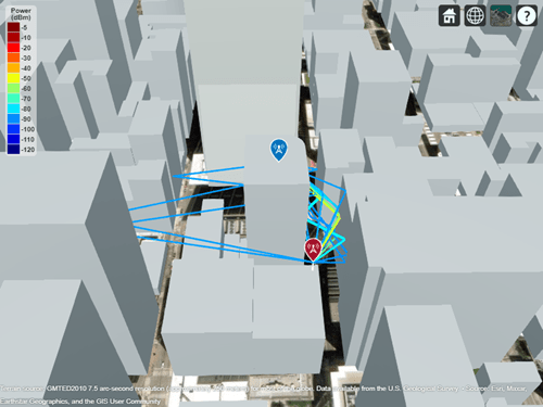
The updated ray tracing model shows more propagation paths from the transmitter to the receiver.
Appendix
[1] The OpenStreetMap file is downloaded from https://www.openstreetmap.org, which provides access to crowd-sourced map data all over the world. The data is licensed under the Open Data Commons Open Database License (ODbL), https://opendatacommons.org/licenses/odbl/.
Launch Site Viewer with buildings in Chicago. For more information about the OpenStreetMap® file, see [1].
viewer = siteviewer(Buildings="chicago.osm");Create a transmitter site on a building and a receiver site near another building.
tx = txsite(Latitude=41.8800, ...
    Longitude=-87.6295, ...
    TransmitterFrequency=2.5e9);
show(tx)
Create a ray tracing propagation model, which MATLAB® represents using a RayTracing object. Configure the model to find paths with up to 2 surface reflections and up to 1 edge diffraction. By default, the model uses the SBR method.
pm = propagationModel("raytracing", ...
    MaxNumReflections=2,MaxNumDiffractions=1);
Display the coverage map.
coverage(tx,pm,SignalStrengths=-100:5)

Appendix
[1] The OpenStreetMap file is downloaded from https://www.openstreetmap.org, which provides access to crowd-sourced map data all over the world. The data is licensed under the Open Data Commons Open Database License (ODbL), https://opendatacommons.org/licenses/odbl/.
Ray tracing models enable you to discard propagation paths based on path loss thresholds.
Specify a threshold relative to the strongest propagation path by using the
MaxRelativePathLossproperty.Specify an absolute threshold by using the
MaxAbsolutePathLossproperty.
Create a Site Viewer with buildings in Chicago. For more information about the OpenStreetMap® file, see [1].
viewer = siteviewer(Buildings="chicago.osm");Create a transmitter site on a building and a receiver site near another building.
tx = txsite(Latitude=41.8800, ...
    Longitude=-87.6295, ...
    TransmitterFrequency=2.5e9);
show(tx)
rx = rxsite(Latitude=41.8813452, ...
    Longitude=-87.629771, ...
    AntennaHeight=30);
show(rx)
Create a ray tracing propagation model, which MATLAB represents using a RayTracing object. Configure the model to find paths with up to 2 surface reflections and up to 1 edge diffraction. By default, the model uses the SBR method.
pm = propagationModel("raytracing", ...
    MaxNumReflections=2, ...
    MaxNumDiffractions=1);
Perform the ray tracing analysis. By default, the model discard paths that are more than 40 dB weaker than the strongest path.
raytrace(tx,rx,pm,Type="pathloss")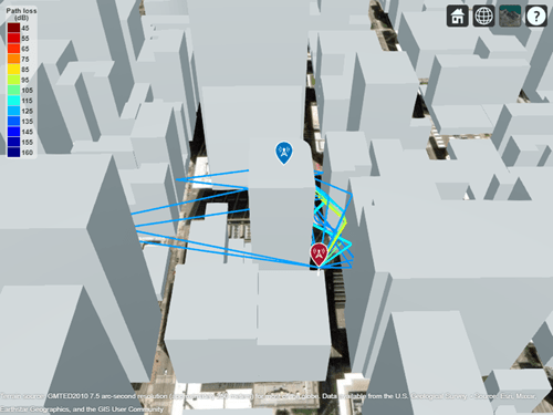
Discard Paths Based on Relative Path Loss
Discard paths that are more than 50 dB weaker than the strongest path by changing the MaxRelativePathLoss property of the RayTracing object. Then, perform the ray tracing analysis again.
pm.MaxRelativePathLoss = 50;
raytrace(tx,rx,pm,Type="pathloss")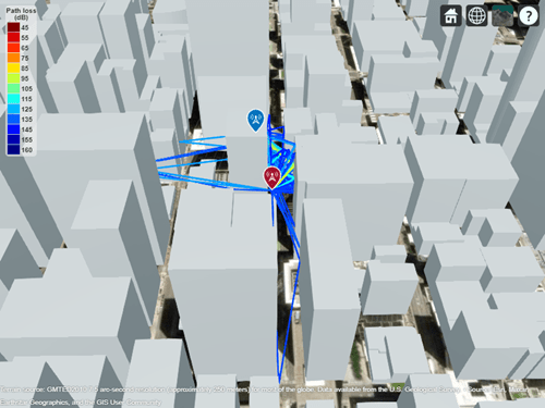
To avoid discarding propagation paths, set the MaxRelativePathLoss property to Inf.
pm.MaxRelativePathLoss = Inf;
raytrace(tx,rx,pm,Type="pathloss")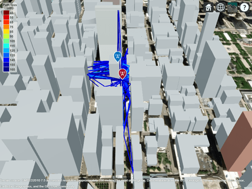
Discard Paths Based on Absolute Path Loss
Discard paths with more than 115 dB of path loss by setting the MaxAbsolutePathLoss property of the RayTracing object.
pm.MaxAbsolutePathLoss = 115;
raytrace(tx,rx,pm,Type="pathloss")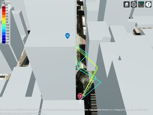
Appendix
[1] The OpenStreetMap file is downloaded from https://www.openstreetmap.org, which provides access to crowd-sourced map data all over the world. The data is licensed under the Open Data Commons Open Database License (ODbL), https://opendatacommons.org/licenses/odbl/.
More About
The shooting and bouncing rays (SBR) method finds an approximate number of propagation paths with exact geometric accuracy. You can use this method to find paths with up to 100 path reflections.
The computational complexity of the SBR method increases linearly with the number of reflections and exponentially with the number of diffractions. The SBR method is generally faster than the image method.
This figure illustrates the SBR method for calculating propagation paths from a transmitter, Tx, to a receiver, Rx.
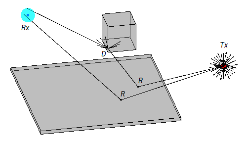
The SBR method launches many rays from a geodesic sphere centered at Tx. The geodesic sphere enables the model to launch rays that are approximately uniformly spaced.
Then, the method traces every ray from Tx and can model different types of interactions between the rays and surrounding objects, such as reflections and diffractions. Note that the current implementation of the SBR method considers only reflections and edge diffractions. In addition, the implementation considers edges for diffraction when the intersection angle for two surfaces is in the range [0.1, 179.9), in degrees.
When a ray hits a flat surface, shown as R, the ray reflects based on the law of reflection.
When a ray hits an edge, shown as D, the ray spawns many diffracted rays based on the law of diffraction [3][4]. Each diffracted ray has the same angle with the diffracting edge as the incident ray. The diffraction point then becomes a new launching point and the SBR method traces the diffracted rays in the same way as the rays launched from Tx. A continuum of diffracted rays forms a cone around the diffracting edge, which is commonly known as a Keller cone [4].
For each launched ray, the SBR method surrounds Rx with a sphere, called a reception sphere, with a radius that is proportional to the distance the ray travels and the average number of degrees between the launched rays. If the ray intersects the sphere, then the model considers the ray a valid path from Tx to Rx. The SBR method corrects the valid paths so that the paths have exact geometric accuracy.
When you increase the number of rays by decreasing the number of degrees between rays, the reception sphere becomes smaller. As a result, in some cases, launching more rays results in fewer or different paths. This situation is more likely to occur with custom 3-D scenarios created from STL files or triangulation objects than with scenarios that are automatically generated from OpenStreetMap buildings and terrain data.
The SBR method finds paths using double-precision floating-point computations.
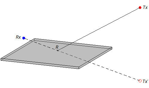
The image method finds an exact number of propagation paths with exact geometric accuracy. You can use this method to find paths with up to 2 path reflections. The computational complexity of the image method increases exponentially with the number of reflections.
This figure illustrates the image method for calculating the propagation path of a single reflection ray for the same transmitter and receiver as the SBR method. The image method locates the image of Tx with respect to a planar reflection surface, Tx'. Then, the method connects Tx' and Rx with a line segment. If the line segment intersects the planar reflection surface, shown as R in the figure, then a valid path from Tx to Rx exists. The method determines paths with multiple reflections by recursively extending these steps. The image method finds paths using single-precision floating-point computations.
Tips
By default, functions that accept a
RayTracingobject as input use terrain elevation data hosted by MathWorks® and derived from the GMTED2010 model by the USGS and NGA. To use terrain elevation data from DTED files instead, first add the terrain by using theaddCustomTerrainfunction. Then, use the terrain by specifying theTerrainproperty of asiteviewerobject or by specifying theMapargument of a propagation function such assigstrengthorsinr.The
comm.Rayobjects created by theraytracefunction calculate path loss using patterns from the antenna arrays stored in theAntennaproperties of the inputtxsiteandrxsiteobjects. By default,RayTracingobjects discard propagation paths based on path loss by using theMaxAbsolutePathLossandMaxRelativePathLossproperties. As a result, when the antennas are polarized, theraytracefunction might unexpectedly discard somecomm.Rayobjects. You can investigate additional propagation paths by setting theAntennaproperty of thetxsiteandrxsiteobjects to"isotropic"or by setting theMaxRelativePathLossproperty of theRayTracingobject toInf.
References
[1] Yun, Zhengqing, and Magdy F. Iskander. “Ray Tracing for Radio Propagation Modeling: Principles and Applications.” IEEE Access 3 (2015): 1089–1100. https://doi.org/10.1109/ACCESS.2015.2453991.
[2] Schaubach, K.R., N.J. Davis, and T.S. Rappaport. “A Ray Tracing Method for Predicting Path Loss and Delay Spread in Microcellular Environments.” In [1992 Proceedings] Vehicular Technology Society 42nd VTS Conference - Frontiers of Technology, 932–35. Denver, CO, USA: IEEE, 1992. https://doi.org/10.1109/VETEC.1992.245274.
[3] International Telecommunications Union Radiocommunication Sector. Propagation by diffraction. Recommendation P.526-15. ITU-R, approved October 21, 2019. https://www.itu.int/rec/R-REC-P.526/en.
[4] Keller, Joseph B. “Geometrical Theory of Diffraction.” Journal of the Optical Society of America 52, no. 2 (February 1, 1962): 116. https://doi.org/10.1364/JOSA.52.000116.
Extended Capabilities
Version History
Introduced in R2019bSee Also
Functions
propagationModel|raytrace|coverage|sigstrength|buildingMaterialPermittivity|earthSurfacePermittivity