Guidance and troubleshooting for parameter estimation in SimBiology
We are often asked to help with parameter estimation problems. This discussion aims to provide guidance for parameter estimation, as well as troubleshooting some of the more common failure modes. We welcome your thoughts and advice in the comments below.
Guidance and Best Practices:
1. Make sure your data is formatted correctly. Your data should have:
- a time column (defined as independent variable) that is monotonically increasing within every grouping variable,
- one or more concentration columns (dependent variable),
- one or more dose columns (with associated rate, if applicable) if you want your model to be perturbed by doses,
- a column with a grouping variable is optional.
Note: the dose column should only have entries at time points where a dose is administered. At time points where the dose is not administered, there should be no entry. When importing your data, MATLAB/SimBiology will replace empty cells with NaNs. Similarly, the concentration column should only have entries where measurements have been acquired and should be left empty otherwise.
If you import your data first in MATLAB, you can manipulate your data into the right format using datatype ' table ' and its methods such as sortrows , join , innerjoin , outerjoin , stack and unstack . You can then add the data to SimBiology by using the 'Import data from MATLAB workspace' functionality.
2. Visually inspect data and model response. Create a simulation task in the SimBiology desktop where you plot your data ( plot external data ), together with your model response. You can create sliders for the parameters you are trying to estimate (or use group simulation). You can then see whether, by varying these parameter values, you can bring the model response in line with your data, while at the same time giving you good initial estimates for those parameters. This plot can also indicate whether units might cause a discrepancy between your simulations and data, and/or whether doses administered to the model are configured correctly and result in a model response.
3. Determine sensitivity of your model response to model parameters. The previous section can be considered a manual sensitivity analysis. There is also a more systematic way of performing such an analysis: a global or local sensitivity analysis can be used to determine how sensitive your responses are to the parameters you are trying to estimate. If a model is not sensitive to a parameter, the parameter’s value may change significantly but this does not lead to a significant change in the model response. As a result, the value of the objective function is not sensitive to changes in that parameter value, hindering estimating the parameter’s value effectively.
4. Choose an optimization algorithm. SimBiology supports a range of optimization algorithms, depending on the toolboxes you have installed. As a default, we would recommend using lsqnonlin if you have access to the Optimization Toolbox. See troubleshooting below for more considerations choosing an appropriate optimization algorithm.
5. Map your data to your model components: Make sure the columns for your dependent variable(s) and dose(s) are mapped to the corresponding component(s) in your model.
6. Start small: bring the estimation task down to the smallest meaningful objective. If you want to estimate 10 parameters, try to start with estimating one or two instead. This will make troubleshooting easier. Once your estimation is set up properly with a few parameters, you can increase the number of parameters.
Troubleshooting
1. Are you trying to estimate a parameter that is governed by a rule? You can’t estimate parameters that are the subject of a rule (initial/repeated assignment, algebraic rule, rate rule), as the rule would supersede the value of the parameter you are trying to estimate. See this topic.
2. Is the optimization using the correct initial conditions and parameter values? Check whether - for the fit task - the parameter values and initial conditions that are used for the model, make sense. You can do this by passing the relevant dose(s) and variant(s) to the getequations function. In the SimBiology App, you can look at your equation view (When you have your model open, in the Model Tab, click Open -> Equations). Subsequently, - in the Model tab - click "Show Tasks" and select your fit task and inspect the initial conditions for your parameters and species. A typical example of this is when you do a dosing species but ka (the absorption rate) is set to zero. In that case, your dose will not transfer into the model and you will not see a model response.
3. Are your units consistent between your data and your model? You can use unit conversion to automatically achieve this.
4. Have you checked your solver tolerances? The absolute and relative tolerance of your solver determine how accurate your model simulation is. If a state in your model is on the order of 1e-9 but your tolerances only allow you to calculate this state with an accuracy down to 1e-8, your state will practically represent a random error around 1e-8. This is especially relevant if your data is on an order that is lower than your solver tolerances. In that case, your objective function will only pick up the solver error, rather than the true model response and will not be able to effectively estimate parameters. When you plot your data and model response together and by using a log-scale on the y-axis (right-click on your Live plot, select Properties, select Axes Properties, select Log scale under “Y-axis”) you can also see whether your ODE solver tolerances are sufficiently small to accurately compute model responses at the order of magnitude of your data. A give-away that this is not the case is when your model response appears to randomly vary as it bottoms-out around absolute solver tolerance.
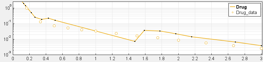
_ Tolerances are too low to simulate at the order of magnitude of the data. Absolute Tolerance: 0.001, Relative Tolerance: 0.01_
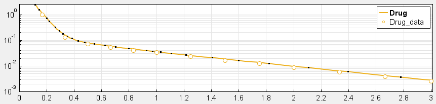
_ Sufficiently high tolerances. Absolute Tolerance: 1e-8, Relative Tolerance: 1e-5_
5. Have you checked the tolerances and stopping criteria of your optimization algorithm? The goal for your optimization should be that it terminates because it meets the imposed tolerances rather than because it exceeds the maximum number of iterations. Optimization algorithms terminate the estimation based on tolerances and stopping criteria. An example of a tolerance here is that you specify the precision with which you want to estimate a certain parameter, e.g. Cl with a precision down to 0.1 ml/hour. If these tolerances and stopping criteria are not set properly, your optimization could terminate early (leading to loss of precision in the estimation) or late (leading to unnecessarily long optimization compute times).
6. Have you considered structural and practical identifiability of your parameters? In your model, there might exist values for two (or more) parameters that result in a very similar model response. When estimating these parameters, the objective function will be very similar for these two parameters, resulting in the optimization algorithm not being able to find a unique set of parameter estimates. This effect is sometimes called aliasing and is a structural identifiability problem. An example would be if you have parallel enzymatic (Km, Vm) and linear clearance (Cl) routes. Practical identifiability occurs when there is not enough data available to sufficiently constrain the parameters you are estimating. An example is estimating the intercompartmental clearance (Q12), when you only have data on the central compartment of a two-compartment model. Another example would be that your data does not capture the process you are trying to estimate, e.g. you don’t have data on the absorption phase but are trying to estimate the absorption constant (Ka).
7. Have you considered trying another optimization algorithm? SimBiology supports a range of optimization algorithms, depending on the toolboxes you have installed. There is no single answer as to which algorithm you should use but some general guidelines can help in selecting the best algorithm.
- Non-linear regression: If your aim is to estimate parameters estimates for each group in your dataset (unpooled) or for all groups (pooled), you can use non-linear regression estimation methods. The optimization algorithms can be broken down into local and global optimization algorithms. You can use a local optimization algorithm when you have good initial estimates for the parameters you are trying to estimate. Each of the local optimization functions has a different default optimization algorithm: fminsearch (Nelder-Mead/downhill simplex search method), fmincon (interior-point), fminunc (quasi-newton), nlinfit (Levenberg-Marquardt), lsqcurvefit, lsqnonlin (both trust-region-reflective algorithm). As a default, we would recommend using lsqnonlin if you have access to the Optimization Toolbox. Note that all but the fminsearch algorithm are gradient based. If a gradient based algorithm fails to find suitable estimates, you can try fminsearch and see whether that improves the optimization. All local optimization algorithms can get “stuck” in a local minimum of the objective function and might therefore fail to reach the true minimum. Global optimization algorithms are developed to find the absolute minimum of the objective function. You can use global optimization algorithms when your fitting task results in different parameter estimates when repeated with different initial values (in other words, your optimization is getting stuck in local minima). You are more likely to encounter this as you increase the number of parameters you are estimating, as you increase the parameter space you are exploring (in other words, the bounds you are imposing on your estimates) and when you have poor initial estimates (in other words, your initial estimates are potentially very far from the estimates that correspond with the minimum of the objective function). A disadvantage of global optimization algorithms is that these algorithms are much more computationally expensive – they often take significantly more time to converge than the local optimization methods do. When using global optimization methods, we recommend using SimBiology’s built-in scattersearch algorithm, combined with lsqnonlin as a local solver. If you have access to the Global Optimization Toolbox, you can try the functions ga (genetic algorithm), patternsearch and particleswarm. Note that some of the global optimization algorithms, including scattersearch, lend themselves well to be accelerated using parallel or distributed computing.
- Estimate category-specific parameters: If you want to estimate category-specific parameters for multiple subjects, e.g. you have 10 male and 10 female subjects in your dataset and you want to estimate a separate clearance value for each gender while all other parameters will be gender-independent, you can also use non-linear regression. Please refer to this example in the documentation.
- Non-linear mixed effects: If your data represents a population of individuals where you think there could be significant inter-individual variability you can use mixed effects modeling to estimate the fixed and random effects present in your population, while also understanding covariance between different parameters you are trying to estimate. When performing mixed effects estimation, it is advisable to perform fixed effects estimation in order to obtain reasonable initial estimates for the mixed effects estimation. SimBiology supports two estimation functions: nlmefit (LME, RELME, FO or FOCE algorithms), and nlmefitsa (Stochastic Approximation Expectation-Maximization). Sometimes, these solvers might seem to struggle to converge. In that case, it is worthwhile determining whether your (objective) function tolerance is set too low and increasing the tolerance somewhat.
8. Does your optimization get stuck? Sometimes, the optimization algorithm can get stuck at a certain iteration. For a particular iteration, the parameter values that model is simulated with as part of the optimization process, can cause the model to be in a state where the ODE solver needs to take very small time-steps to achieve the tolerances (e.g. very rapid changes of model responses). Solutions can include: changing your initial estimates, imposing lower and upper bounds on the parameters you are trying to estimate, selecting to a different solver, easing solver tolerances (only where possible, see also “Visually inspect data and model response”).
9. Are you using the proportional error model? The objective function for the proportional error model contains a term where your response data is part of the denominator. As response variables get close to zero or are exactly zero, this effectively means the objective function contains one or more terms that divide by zero, causing errors or at least very slow iterations of your optimization algorithm. You can try to change the error model to constant or combined to circumvent this problem. Alternatively, you can define separate error models for each response: proportional for those responses that don’t have measurements that contain values close to zero and a constant error model for those responses that do.
1 Kommentar
Zeit (absteigend)Excellent points and a very well-written article which I am sure many would find useful!