Ergebnisse für
Title: Looking for Internship Guidance as a Beginner MATLAB/Simulink Learner
Hello everyone,
I’m a Computer Science undergraduate currently building a strong foundation in MATLAB and Simulink. I’m still at a beginner level, but I’m actively learning every day and can work confidently once I understand the concepts. Right now I’m focusing on MATLAB modeling, physics simulation, and basic control systems so that I can contribute effectively to my current project.
I’m part of an Autonomous Underwater Vehicle (AUV) team preparing for the Singapore AUV Challenge (SAUVC). My role is in physics simulation, controls, and navigation, and MATLAB/Simulink plays a major role in that pipeline. I enjoy physics and mathematics deeply, which makes learning modeling and simulation very exciting for me.
On the coding side, I practice competitive programming regularly—
• Codeforces rating: ~1200
• LeetCode rating: ~1500
So I'm comfortable with logic-building and problem solving. What I’m looking for:
I want to know how a beginner like me can start applying for internships related to MATLAB, Simulink, modeling, simulation, or any engineering team where MATLAB is widely used (including companies outside MathWorks).
I would really appreciate advice from the community on:
- What skills should I strengthen first?
- Which MATLAB/Simulink toolboxes are most important for beginners aiming toward simulation/control roles?
- What small projects or portfolio examples should I build to improve my profile?
- What is the best roadmap to eventually become a good candidate for internships in this area?
Any guidance, resources, or suggestions would be extremely helpful for me.
Thank you in advance to everyone who shares their experience!
Jorge Bernal-AlvizJorge Bernal-Alviz shared the following code that requires R2025a or later:
Test()
function Test()
duration = 10;
numFrames = 800;
frameInterval = duration / numFrames;
w = 400;
t = 0;
i_vals = 1:10000;
x_vals = i_vals;
y_vals = i_vals / 235;
r = linspace(0, 1, 300)';
g = linspace(0, 0.1, 300)';
b = linspace(1, 0, 300)';
r = r * 0.8 + 0.1;
g = g * 0.6 + 0.1;
b = b * 0.9 + 0.1;
customColormap = [r, g, b];
figure('Position', [100, 100, w, w], 'Color', [0, 0, 0]);
axis equal;
axis off;
xlim([0, w]);
ylim([0, w]);
hold on;
colormap default;
colormap(customColormap);
plothandle = scatter([], [], 1, 'filled', 'MarkerFaceAlpha', 0.12);
for i = 1:numFrames
t = t + pi/240;
k = (4 + 3 * sin(y_vals * 2 - t)) .* cos(x_vals / 29);
e = y_vals / 8 - 13;
d = sqrt(k.^2 + e.^2);
c = d - t;
q = 3 * sin(2 * k) + 0.3 ./ (k + 1e-10) + ...
sin(y_vals / 25) .* k .* (9 + 4 * sin(9 * e - 3 * d + 2 * t));
points_x = q + 30 * cos(c) + 200;
points_y = q .* sin(c) + 39 * d - 220;
points_y = w - points_y;
CData = (1 + sin(0.1 * (d - t))) / 3;
CData = max(0, min(1, CData));
set(plothandle, 'XData', points_x, 'YData', points_y, 'CData', CData);
brightness = 0.5 + 0.3 * sin(t * 0.2);
set(plothandle, 'MarkerFaceAlpha', brightness);
drawnow;
pause(frameInterval);
end
end
Parallel Computing Onramp is here! This free, one-hour self-paced course teaches the basics of running MATLAB code in parallel using multiple CPU cores, helping users speed up their code and write code that handles information efficiently.
Remember, Onramps are free for everyone - give the new course a try if you're curious. Let us know what you think of it by replying below.
I am excited to join this community to learn the more particularly the Matlab/Simulink
I'm developing a comprehensive MATLAB programming course and seeking passionate co-trainers to collaborate!
Why MATLAB Matters:Many people underestimate MATLAB's significance in:
- Communication systems
- Signal processing
- Mathematical modeling
- Engineering applications
- Scientific computing
Course Structure:
- Foundation Module: MATLAB basics and fundamentals
- Image Processing: Practical applications and techniques
- Signal Processing: Analysis and implementation
- Machine Learning: ML algorithms using MATLAB
- Hands-on Learning: Projects, assignments.
What I'm Looking For:
- Enthusiastic educators willing to share knowledge
- Experience in any MATLAB application area
- Commitment to collaborative teaching
Interested in joining as a co-trainer? Please comment below or reach out directly!
Online Doc + System Browser
11%
Online Doc + Dedicated Browser
11%
Offline Doc +System Browser
11%
Offline Doc + Dedicated Browser
23%
Hybrid Approach (Support All Modes)
23%
User-Definable / Fully Configurable
20%
35 Stimmen
Inspired by @xingxingcui's post about old MATLAB versions and @유장's post about an old Easter egg, I thought it might be fun to share some MATLAB-Old-Timer Stories™.
Back in the early 90s, MATLAB had been ported to MacOS, but there were some interesting wrinkles. One that kept me earning my money as a computer lab tutor was that MATLAB required file names to follow Windows standards - no spaces or other special characters. But on a Mac, nothing stopped you from naming your script "hello world - 123.m". The problem came when you tried to run it. MATLAB was essentially doing an eval on the script name, assuming the file name would follow Windows (and MATLAB) naming rules.
So now imagine a lab full of students taking a university course. As is common in many universities, the course was given a numeric code. For whatever historical reason, my school at that time was also using numeric codes for the departments. Despite being told the rules for naming scripts, many students would default to something like "26.165 - 1.1" for problem one on HW1 for the intro applied math course 26.165.
No matter what they did in their script, when they ran it, MATLAB would just say "ans = 25.0650".
Nothing brings you more MATLAB-god credibility as a student tutor than walking over to someone's computer, taking one look at their output, saying "rename your file", and walking away like a boss.
I recently published this blog post about resources to help people learn MATLAB https://blogs.mathworks.com/matlab/2025/09/11/learning-matlab-in-2025/
What are your favourite MATLAB learning resources?
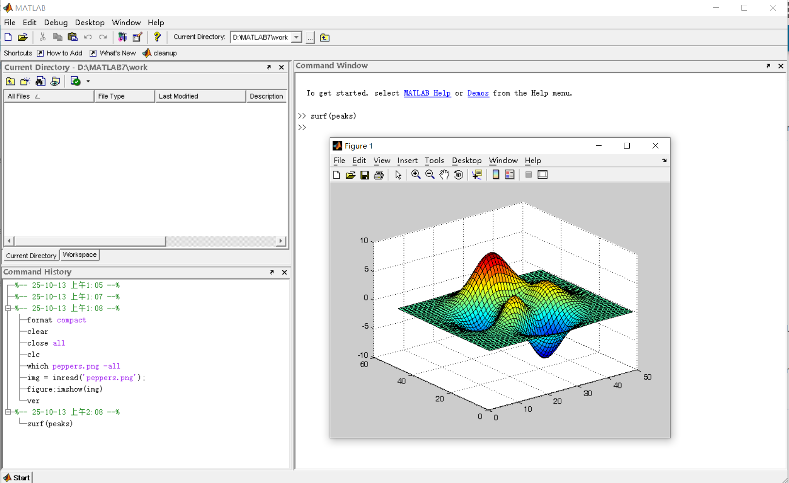
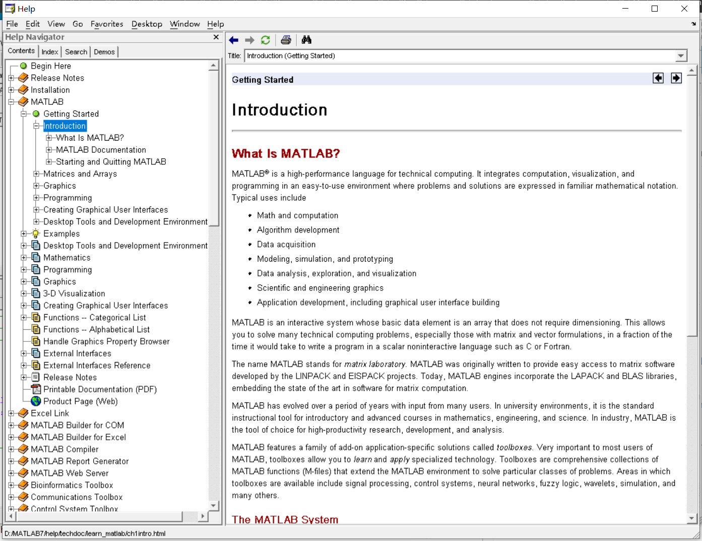
It was 2010 when I was a sophomore in university. I chose to learn MATLAB because of a mathematical modeling competition, and the university provided MATLAB 7.0, a very classic release. To get started, I borrowed many MATLAB books from the library and began by learning simple numerical calculations, plotting, and solving equations. Gradually I was drawn in by MATLAB’s powerful capabilities and became interested; I often used it as a big calculator for fun. That version didn’t have MATLAB Live Script; instead it used MATLAB Notebook (M-Book), which allowed MATLAB functions to be used directly within Microsoft Word, and it also had the Symbolic Math Toolbox’s MuPAD interactive environment. These were later gradually replaced by Live Scripts introduced in R2016a. There are many similar examples...
Out of curiosity, I still have screenshots on my computer showing MATLAB 7.0 running compatibly. I’d love to hear your thoughts?


Share your learning starting trouble experience of Matlab.. Looking forward for more answers..
Helllo all
I write The MATLAB Blog and have covered various enhancements to MATLAB's ODE capabilities over the last couple of years. Here are a few such posts
- The new solution framework for Ordinary Differential Equations (ODEs) in MATLAB R2023b
- Faster Ordinary Differential Equations (ODEs) solvers and Sensitivity Analysis of Parameters: Introducing SUNDIALS support in MATLAB
- Solving Higher-Order ODEs in MATLAB
- Function handles are faster in MATLAB R2023a (Faster function handles led to faster ode45 and friends)
- Understanding Tolerances in Ordinary Differential Equation Solvers
Everyone in this community has deeply engaged with all of these posts and given me lots of ideas for future enhancements which I've dutifully added to our internal enhancment request database.
Because I've asked for so much in this area, I was recently asked if there's anything else we should consider in the area of ODEs. Since all my best ideas come from all of you, I'm asking here....
So. If you could ask for new and improved functionality for solving ODEs with MATLAB, what would it be and (ideally) why?
Cheers,
Mike
Yesterday I had an urgent service call for MatLab tech support. The Mathworks technician on call, Ivy Ngyuen, helped fix the problem. She was very patient and I truly appreciate her efforts, which resolved the issue. Thank you.

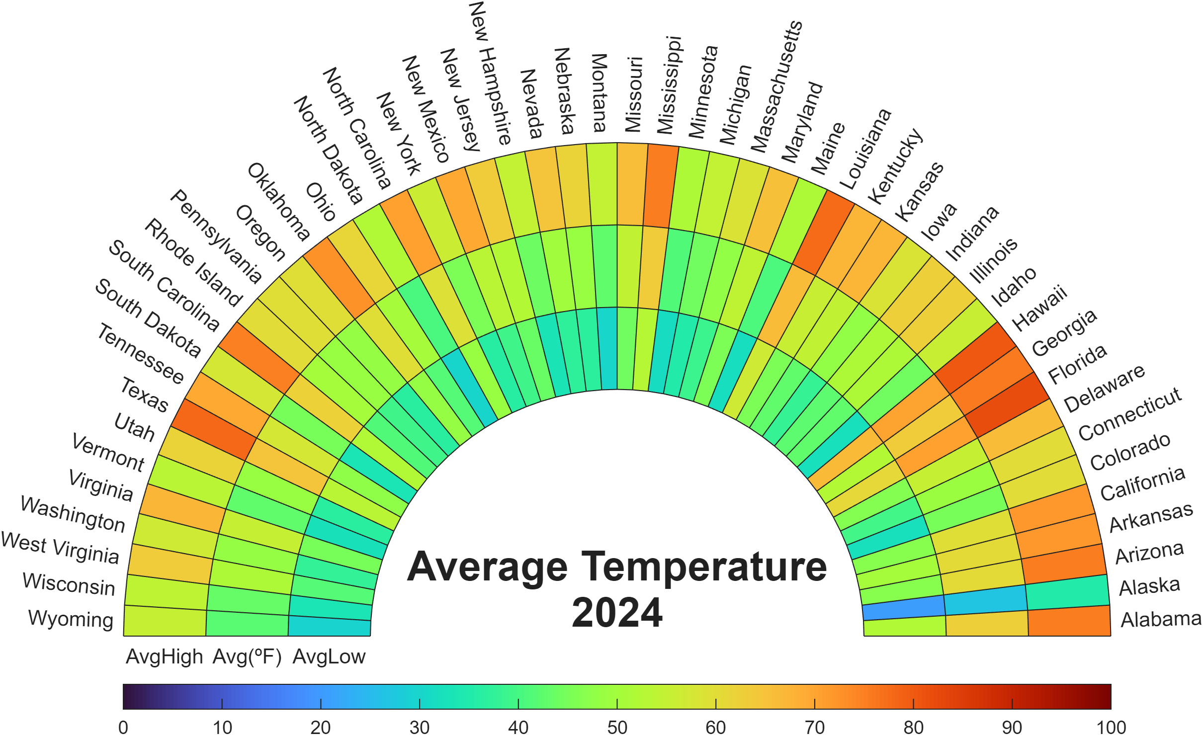
Check out how these charts were made with polar axes in the Graphics and App Building blog's latest article "Polar plots with patches and surface".

Nine new Image Processing courses plus one new learning path are now available as part of the Online Training Suite. These courses replace the content covered in the self-paced course Image Processing with MATLAB, which sunsets in 2026.
New courses include:
- Work with Image Data Types
- Image Registration
- Edge, Circle, and Line Detection
- Manage and Process Multiple Images
The new learning path Image Segmentation and Analysis in MATLAB earns users the digital credential Image Segmentation in MATLAB and contains the following courses:
Do you have a swag signed by Brian Douglas? He does!
Apparently, the back end here is running 2025b, hovering over the Run button and the Executing In popup both show R2024a.
ver matlab
all(logical.empty)
Discuss!
I just noticed that MATLAB R2025b is available. I am a bit surprised, as I never got notification of the beta test for it.
This topic is for highlights and experiences with R2025b.
