Parasite Classification Using Wavelet Scattering and Deep Learning
This example shows how to classify parasitic infections in Giemsa stain images using wavelet image scattering and deep learning. The data set is challenging for deep networks because it contains only 48 images. The images are divided evenly into three categories of parasitic infections: babesiosis, plasmodium-gametocyte, and trypanosomiasis.
Data
Unzip the BloodSmearImages.zip file into a folder where you have write permission. This example uses the directory corresponding to the value of tempdir in MATLAB®. To use another folder, set dataFolder equal to that value in the following code.
dataFolder = tempdir;
unzip("BloodSmearImages.zip",dataFolder);
In the BloodSmearImages folder, you can find a README.txt file that details the original source of all images.
Create an ImageDatastore to manage the access of the Giemsa stain images. The images are in RGB format with a common size of 300-by-300-by-3.
imagedir = fullfile(dataFolder,"BloodSmearImages");
imds = imageDatastore(imagedir,IncludeSubFolders=true, ...
    FileExtensions=".jpg",LabelSource="foldernames");
summary(imds.Labels,Statistics="counts")
48×1 categorical

     babesiosis                 16
     plasmodium-gametocyte      16
     trypanosomiasis            16
There are 16 images for each of the three parasite types. Split the data into training and hold-out test sets, with 70 percent of the images in the training set and 30 percent in the test set. Set the random number generator for reproducibility.
rng default
[imdsTrain,imdsTest] = splitEachLabel(imds,0.7);
Verify that equal numbers of each parasite class are contained in both the training and test sets.
summary(imdsTrain.Labels,Statistics="counts")33×1 categorical
babesiosis 11
plasmodium-gametocyte 11
trypanosomiasis 11
% Perform the same for the test set.
summary(imdsTest.Labels,Statistics="counts")
15×1 categorical

     babesiosis                 5
     plasmodium-gametocyte      5
     trypanosomiasis            5
Because this is a small data set, the entire training and test sets fit in memory. Read all images for both sets.
trainImages = readall(imdsTrain);
testImages = readall(imdsTest);
Plot some sample images from the training data.
idx = randperm(33,6);
tiledlayout(3,2)
for ii = 1:length(idx)
    im = trainImages{idx(ii)};
    nexttile
    imshow(im,[])
    title(string(imdsTrain.Labels(idx(ii))));
end

Wavelet Scattering Network
In this example, you use a wavelet scattering transform as the feature extractor for the machine learning approaches. The wavelet scattering transform helps to reduce the dimensionality of the data and increase the interclass dissimilarity. Construct a two-layer image scattering network with a 40-by-40 pixel invariance scale. Use two wavelets per octave in the first layer and one wavelet per octave in the second layer. Use two rotations of the wavelets per layer.
sn = waveletScattering2(ImageSize=[300 300],InvarianceScale=40, ...
    QualityFactors=[2 1],NumRotations=[2 2]);
[~,npaths] = paths(sn);
sum(npaths)
ans = 27
coefficientSize(sn)
ans = 1×2

    38    38
The specified wavelet scattering network has 27 paths. The image on each scattering path is reduced to 38-by-38-by-3. Even without further averaging of the scattering coefficients, this is a reduction in the size of each image's memory by more than a factor of 2. However, for classification we form a feature vector that averages the scattering coefficients over the spatial and channel dimensions. This results in feature vectors with only 27 elements, a real-valued scalar for each scattering path. This represents a reduction in the number of elements by a factor of 10,000 for each image.
The following code computes the wavelet scattering feature vectors for both the training and test sets. Concatenate the feature vectors so that you have N-by-27 matrices, where N is the number of examples in the training or test set and each row is a wavelet scattering feature vector for an example.
trainfeatures = cellfun(@(x)helperScatImages_mean(sn,x),trainImages,UniformOutput=false);
testfeatures = cellfun(@(x)helperScatImages_mean(sn,x),testImages,UniformOutput=false);
trainfeatures = cat(1,trainfeatures{:});
testfeatures = cat(1,testfeatures{:});
SVM Classification
Use an SVM classifier with the scattering features. Choose a cubic polynomial kernel. Use a one-vs-all coding scheme.
template = templateSVM(...
    KernelFunction="polynomial", ...
    PolynomialOrder=3, ...
    KernelScale=1, ...
    BoxConstraint=314, ...
    Standardize=true);
classificationSVM = fitcecoc(trainfeatures,imdsTrain.Labels, ...
    Learners=template,Coding="onevsall");
Estimate the accuracy on the training set using cross-validation with 5 folds.
kfoldmodel = crossval(classificationSVM,KFold=5);
loss = kfoldLoss(kfoldmodel)*100;
crossvalAccuracy = 100-loss
crossvalAccuracy = single

81.8182
The cross-validation accuracy is approximately 80 percent. Now examine the accuracy on the held-out test set and plot the confusion chart.
predLabels = predict(classificationSVM,testfeatures);
testAccuracy = ...
    sum(categorical(predLabels)==imdsTest.Labels)/numel(imdsTest.Labels)*100
testAccuracy = 80
figure
cchart = confusionchart(imdsTest.Labels,predLabels);
cchart.Title = ...
    {"Confusion Chart for Wavelet";"Scattering Features Using SVM"};
cchart.RowSummary = "row-normalized";
cchart.ColumnSummary = "column-normalized";
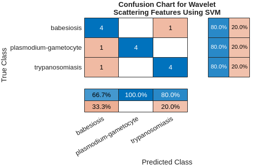
The overall test accuracy is also approximately 80 percent with the SVM model. The recall for each class is 80%. The precision is also good for the plasmodium-gametocyte and trypanosomiasis parasites, but worse for babesiosis. Examine the F1 scores for each class.
f1SVM = f1score(cchart.NormalizedValues);
disp(f1SVM)
                               F1
                             _______

    babesiosis               0.72727
    plasmodium-gametocyte    0.88889
    trypanosomiasis              0.8
All F1 scores are between approximately 0.7 and 0.9.
PCA Classifier with Scattering Features
Support vector machines are powerful techniques for features that are not linearly separable, but they are designed for binary classification and may be suboptimal for multiclass problems. Here you complement the SVM analysis by using a simple PCA (linear) classifier with the same wavelet scattering features. The helperPCAModel function determines the numcomp eigenvectors corresponding to the largest eigenvalues of the covariance matrix of the wavelet scattering features for each pathogen in the training set along with the class means.
helperPCAClassifier classifies each test sample. It does this by subtracting the model class means from each wavelet scattering feature vector in the test data set and projecting the centered feature vectors onto the covariance-matrix eigenvectors for each class in the model. helperPCAClassifier assigns each test example to the pathogen with the smallest error, or residual. This is a principal components analysis (PCA) classifier.
Remove the 0-th order scattering features from each feature vector. Set the number of principal components (eigenvectors) to 6.
numcomp = 6;
model = helperPCAModel(trainfeatures(:,2:end)',numcomp,imdsTrain.Labels);
PCALabels = helperPCAClassifier(testfeatures(:,2:end)',model);
testPCAacc = sum(PCALabels==imdsTest.Labels)/numel(imdsTest.Labels)*100
testPCAacc =
86.6667
The test accuracy is approximately 87% with the PCA classifier. Plot the confusion chart and calculate the F1 scores for each class.
figure
cchart = confusionchart(imdsTest.Labels,PCALabels);
cchart.Title = {"Confusion Chart for Wavelet Scattering Features"; ...
    "Using PCA Classifier"};
cchart.RowSummary = "row-normalized";
cchart.ColumnSummary = "column-normalized";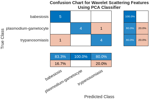
f1PCA = f1score(cchart.NormalizedValues);
disp(f1PCA)
                               F1
                             _______

    babesiosis               0.90909
    plasmodium-gametocyte    0.88889
    trypanosomiasis              0.8
The F1 scores for the PCA classifier with wavelet scattering features are quite strong, with all scores between 0.8 and 1.
Classification Using Deep Convolutional Networks
In this section, you attempt the same classification using deep convolutional networks. Deep networks provide state-of-art results for classification problems with large data sets and are capable of learning complicated nonlinear mappings, but their performance often suffers in small data sets. To mitigate this problem, use an image augmenter. imageDataAugmenter perturbs the data in each epoch, in effect creating new training examples.
augmenter = imageDataAugmenter(RandRotation=[0 180],RandXTranslation=[-5 5], ...
    RandYTranslation=[-5 5]);
augimds = augmentedImageDatastore([300 300 3],imdsTrain,DataAugmentation=augmenter);
Train Simple Convolutional Neural Network
Define a small convolutional neural network (CNN) consisting of two convolution layers followed by batch normalization layers and RELU activations. Follow the final RELU activation with max pooling, fully connected, and softmax layers.
layers = [
imageInputLayer([300 300 3])
convolution2dLayer(7,16)
batchNormalizationLayer
reluLayer
convolution2dLayer(3,20)
batchNormalizationLayer
reluLayer
maxPooling2dLayer(4)
fullyConnectedLayer(3)
softmaxLayer
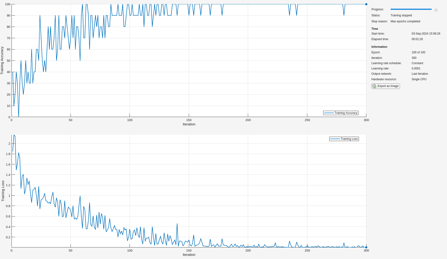
];Use stochastic gradient descent with a mini-batch size of 10. Shuffle the data each epoch. Run the training for 100 epochs. To train on a GPU if one is available, specify the execution environment "auto". Using a GPU requires Parallel Computing Toolbox™ and a supported GPU device. For information on supported devices, see GPU Computing Requirements (Parallel Computing Toolbox).
opts = trainingOptions("sgdm", ...
    InitialLearnRate=0.0001, ...
    MaxEpochs=100, ...
    MiniBatchSize=10, ...
    Shuffle="every-epoch", ...
    Plots="training-progress", ...
    Metrics="accuracy", ...
    Verbose=false, ...
    ExecutionEnvironment="cpu");
Train the neural network using the trainnet (Deep Learning Toolbox) function. For classification, use cross-entropy loss.
trainedNet = trainnet(augimds,layers,"crossentropy",opts);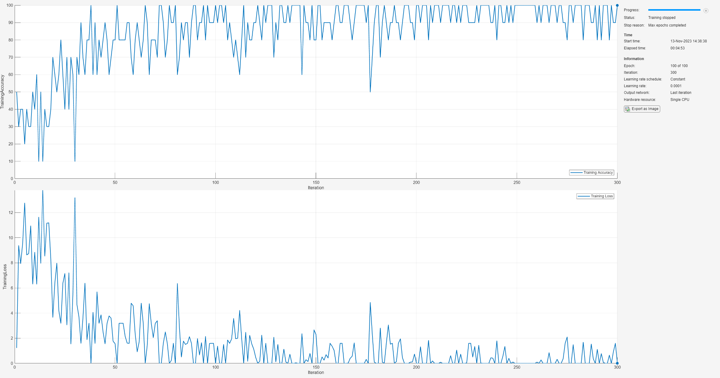
Examine the performance of the network on the held-out test set.
classNames = categories(imdsTrain.Labels);
scores = minibatchpredict(trainedNet,imdsTest);
ypred = scores2label(scores,classNames);
cnnAccuracy = sum(ypred == imdsTest.Labels)/numel(imdsTest.Labels)*100
cnnAccuracy =
60
figure
cchart = confusionchart(imdsTest.Labels,ypred);
cchart.Title = "Confusion Chart for Deep CNN";
cchart.RowSummary = "row-normalized";
cchart.ColumnSummary = "column-normalized";
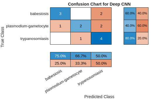
f1CNN = f1score(cchart.NormalizedValues);
disp(f1CNN)
                               F1
                             _______

    babesiosis               0.66667
    plasmodium-gametocyte        0.5
    trypanosomiasis          0.61538
In spite of using an augmented data set for training, the CNN has overfit the training set and the F1 scores are significantly worse than either the SVM or PCA model with the wavelet scattering features.
Transfer Learning with Pretrained SqueezeNet Neural Network
Next, classify the images using transfer learning with a pretrained SqueezeNet neural network.
Load a pretrained SqueezeNet neural network. For a list of all available networks, see Pretrained Deep Neural Networks (Deep Learning Toolbox).
Modify the final convolutional layer to accommodate the fact that you have three classes of pathogens. SqueezeNet was constructed to recognize 1,000 classes.
net = imagePretrainedNetwork("squeezenet");
oldFinalConv = net.Layers(end-4);
numClasses = numel(classNames);
newFinalConv = convolution2dLayer(1,numClasses, ...
        Name="new_conv");
setLearnRateFactor(newFinalConv,Weights=10);
setLearnRateFactor(newFinalConv,Bias=10)
ans =
  Convolution2DLayer with properties:

              Name: 'new_conv'

   Hyperparameters
        FilterSize: [1 1]
       NumChannels: 'auto'
        NumFilters: 3
            Stride: [1 1]
    DilationFactor: [1 1]
       PaddingMode: 'manual'
       PaddingSize: [0 0 0 0]
      PaddingValue: 0

   Learnable Parameters
           Weights: []
              Bias: []

  Show all properties
net = replaceLayer(net,oldFinalConv.Name,newFinalConv);
Reset the training and test datastores. Modify the datastore read function to resize images to be compatible with SqueezeNet, which expects 227-by-227-by-3 images. Set up the image augmenter and train the network.
reset(imdsTrain)
reset(imdsTest)
imdsTrain.ReadFcn = @(x)imresize(imread(x),OutputSize=[227 227]);
imdsTest.ReadFcn = @(x)imresize(imread(x),OutputSize=[227 227]);
augmenter = imageDataAugmenter(RandRotation=[0 180], ...
    RandXTranslation=[-5 5], ...
    RandYTranslation=[-5 5]);
augimds = augmentedImageDatastore([227 227 3],imdsTrain,...
    DataAugmentation=augmenter);
trainedNet = trainnet(augimds,net,"crossentropy",opts);
Obtain the SqueezeNet accuracy, plot the confusion chart, and compute the F1 scores.
classNames = categories(imdsTrain.Labels);
scores = minibatchpredict(trainedNet,imdsTest);
ypred = scores2label(scores,classNames);
sqznetAccuracy = sum(ypred == imdsTest.Labels)/numel(imdsTest.Labels)*100
sqznetAccuracy =
66.6667
figure
cchart = confusionchart(imdsTest.Labels,ypred);
cchart.Title = {"Confusion Chart for Transfer Learning";"with SqueezeNet"};
cchart.RowSummary = "row-normalized";
cchart.ColumnSummary = "column-normalized";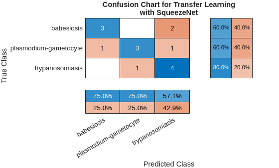
f1SqueezeNet = f1score(cchart.NormalizedValues);
disp(f1SqueezeNet)
                               F1
                             _______

    babesiosis               0.66667
    plasmodium-gametocyte    0.66667
    trypanosomiasis          0.66667
SqueezeNet performance is comparable to the simpler CNN, but its performance does not match the accuracy of the simpler PCA classifier with the wavelet scattering features.
Summary
In this example, the wavelet scattering transform and deep learning frameworks were used to classify pathogens in Giemsa stain images. The limited data set size provides challenges for training a deep learning classifier even when data augmentation is used. The example illustrated that the wavelet scattering transform can provide a useful alternative to deep networks in such cases. In forming feature vectors from the wavelet scattering transform, we reduced each transform output from a 27-by-38-by-38-by-3 tensor to a 27-element vector. Accordingly, we have used a global pooling of the scattering coefficients. It is possible to utilize other pooling schemes, which could yield better results.
Appendix — Supporting Functions
function features = helperScatImages_mean(sn,x)
smat = featureMatrix(sn,x);
features = mean(smat,2:4);
features = features';
end
function F1scores = f1score(cchartVal)
N = sum(cchartVal,'all');
probT = sum(cchartVal)./N;
classProbEst = diag(cchartVal)./N;
Prec = classProbEst'./probT;
probC = [5/15 5/15 5/15];
Recall = classProbEst'./probC;
F1scores = harmmean([Prec ; Recall]);
F1scores = F1scores';
F1scores = table(F1scores,'VariableNames',{'F1'}, ...
    'RowNames',{'babesiosis','plasmodium-gametocyte','trypanosomiasis'});
end

function labels = helperPCAClassifier(features,model)
% This function is only to support wavelet image scattering examples in
% Wavelet Toolbox. It may change or be removed in a future release.
% model is a structure array with fields, M, mu, v, and Labels
% features is the matrix of test data which is Ns-by-L, Ns is the number of
% scattering paths and L is the number of test examples. Each column of
% features is a test example.

labelIdx = determineClass(features,model);
labels = model.Labels(labelIdx);
% Returns as column vector to agree with imageDatastore Labels
labels = labels(:);


%--------------------------------------------------------------------------
function labelIdx = determineClass(features,model)
% Determine number of classes
Nclasses = numel(model.Labels);
% Initialize error matrix
errMatrix = Inf(Nclasses,size(features,2));
for nc = 1:Nclasses
    % class centroid
    mu = model.mu{nc};
    u = model.U{nc};
    % 1-by-L
    errMatrix(nc,:) = projectionError(features,mu,u);
end
% Determine minimum along class dimension
[~,labelIdx] = min(errMatrix,[],1);


%--------------------------------------------------------------------------
function totalerr = projectionError(features,mu,u)
    %
    Npc = size(u,2);
    L = size(features,2);
    % Subtract class mean: Ns-by-L minus Ns-by-1
    s = features-mu;
    % 1-by-L
    normSqX = sum(abs(s).^2,1)';
    err = Inf(Npc+1,L);
	err(1,:) = normSqX;
    err(2:end,:) = -abs(u'*s).^2;
    % 1-by-L
    totalerr = sqrt(sum(err,1));
end
end
end

function model = helperPCAModel(features,M,Labels)
% This function is only to support wavelet image scattering examples in
% Wavelet Toolbox. It may change or be removed in a future release.
% model = helperPCAModel(features,M,Labels)

% Initialize structure array to hold the affine model
model = struct('Dim',[],'mu',[],'U',[],'Labels',categorical([]),'S',[]);
model.Dim = M;
% Obtain the number of classes
LabelCategories = categories(Labels);
Nclasses = numel(categories(Labels));
for kk = 1:Nclasses
    Class = LabelCategories{kk};
    % Find indices corresponding to each class
    idxClass = Labels == Class;
    % Extract feature vectors for each class
    tmpFeatures = features(:,idxClass);
    % Determine the mean for each class
    model.mu{kk} = mean(tmpFeatures,2);
    [model.U{kk},model.S{kk}] = scatPCA(tmpFeatures);
    if size(model.U{kk},2) > M
        model.U{kk} = model.U{kk}(:,1:M);
        model.S{kk} = model.S{kk}(1:M);

    end
    model.Labels(kk) = Class;
end

    function [u,s] = scatPCA(x)
        % Calculate the principal components of x along the second dimension.
        [u,d] = eig(cov(x'));
        % Sort eigenvalues of covariance matrix in descending order
        [s,ind] = sort(diag(d),"descend");
        % sort eigenvector matrix accordingly
        u = u(:,ind);
    end
end