fitgmdist
Fit Gaussian mixture model to data
Description
GMModel = fitgmdist(X,k,Name,Value)Name,Value pair arguments.
For example, you can specify a regularization value or the covariance type.
Examples
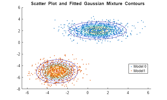
Generate data from a mixture of two bivariate Gaussian distributions.
mu1 = [1 2];
Sigma1 = [2 0; 0 0.5];
mu2 = [-3 -5];
Sigma2 = [1 0;0 1];
rng(1); % For reproducibility
X = [mvnrnd(mu1,Sigma1,1000); mvnrnd(mu2,Sigma2,1000)];
Fit a Gaussian mixture model. Specify that there are two components.
GMModel = fitgmdist(X,2);
Plot the data over the fitted Gaussian mixture model contours.
figure
y = [zeros(1000,1);ones(1000,1)];
h = gscatter(X(:,1),X(:,2),y);
hold on
gmPDF = @(x,y) arrayfun(@(x0,y0) pdf(GMModel,[x0 y0]),x,y);
g = gca;
fcontour(gmPDF,[g.XLim g.YLim])
title('{\bf Scatter Plot and Fitted Gaussian Mixture Contours}')
legend(h,'Model 0','Model1')
hold off

Generate data from a mixture of two bivariate Gaussian distributions. Create a third predictor that is the sum of the first and second predictors.
mu1 = [1 2];
Sigma1 = [1 0; 0 1];
mu2 = [3 4];
Sigma2 = [0.5 0; 0 0.5];
rng(3); % For reproducibility
X1 = [mvnrnd(mu1,Sigma1,100);mvnrnd(mu2,Sigma2,100)];
X = [X1,X1(:,1)+X1(:,2)];
The columns of X are linearly dependent. This can cause ill-conditioned covariance estimates.
Fit a Gaussian mixture model to the data. You can use try / catch statements to help manage error messages.
rng(1); % Reset seed for common start values
try
    GMModel = fitgmdist(X,2)
catch exception
    disp('There was an error fitting the Gaussian mixture model')
    error = exception.message
end
There was an error fitting the Gaussian mixture model
error =
'Ill-conditioned covariance created at iteration 2.'
The covariance estimates are ill-conditioned. Consequently, optimization stops and an error appears.
Fit a Gaussian mixture model again, but use regularization.
rng(3); % Reset seed for common start values
GMModel = fitgmdist(X,2,'RegularizationValue',0.1)
GMModel =

Gaussian mixture distribution with 2 components in 3 dimensions
Component 1:
Mixing proportion: 0.536725
Mean:    2.8831    3.9506    6.8338

Component 2:
Mixing proportion: 0.463275
Mean:    0.8813    1.9758    2.8571
In this case, the algorithm converges to a solution due to regularization.
Gaussian mixture models require that you specify a number of components before being fit to data. For many applications, it might be difficult to know the appropriate number of components. This example shows how to explore the data, and try to get an initial guess at the number of components using principal component analysis.
Load Fisher's iris data set.
load fisheriris
classes = unique(species)
classes = 3×1 cell
{'setosa' }
{'versicolor'}
{'virginica' }
The data set contains three classes of iris species. The analysis proceeds as if this is unknown.
Use principal component analysis to reduce the dimension of the data to two dimensions for visualization.
[~,score] = pca(meas,'NumComponents',2);Fit three Gaussian mixture models to the data by specifying 1, 2, and 3 components. Increase the number of optimization iterations to 1000. Use dot notation to store the final parameter estimates. By default, the software fits full and different covariances for each component.
GMModels = cell(3,1); % Preallocation
options = statset('MaxIter',1000);
rng(1); % For reproducibility

for j = 1:3
    GMModels{j} = fitgmdist(score,j,'Options',options);
    fprintf('\n GM Mean for %i Component(s)\n',j)
    Mu = GMModels{j}.mu
end
GM Mean for 1 Component(s)
Mu = 1×2
10-15 ×

    0.9607   -0.4371
GM Mean for 2 Component(s)
Mu = 2×2

    1.3212   -0.0954
   -2.6424    0.1909
GM Mean for 3 Component(s)
Mu = 3×2

    0.4856   -0.1287
    1.4484   -0.0904
   -2.6424    0.1909
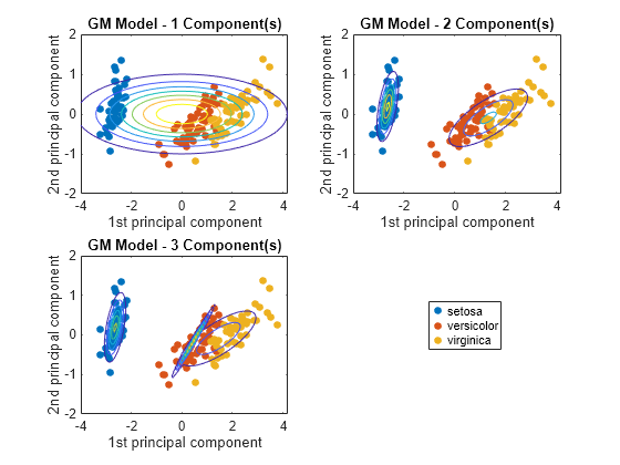
GMModels is a cell array containing three, fitted gmdistribution models. The means in the three component models are different, suggesting that the model distinguishes among the three iris species.
Plot the scores over the fitted Gaussian mixture model contours. Since the data set includes labels, use gscatter to distinguish between the true number of components.
figure
for j = 1:3
    subplot(2,2,j)
    h1 = gscatter(score(:,1),score(:,2),species);
    h = gca;
    hold on
    gmPDF = @(x,y) arrayfun(@(x0,y0) pdf(GMModels{j},[x0 y0]),x,y);
    fcontour(gmPDF,[h.XLim h.YLim],'MeshDensity',100)
    title(sprintf('GM Model - %i Component(s)',j));
    xlabel('1st principal component');
    ylabel('2nd principal component');
    if(j ~= 3)
        legend off;
    end
    hold off
end
g = legend(h1);
g.Position = [0.7 0.25 0.1 0.1];

The three-component Gaussian mixture model, in conjunction with PCA, looks like it distinguishes between the three iris species.
There are other options you can use to help select the appropriate number of components for a Gaussian mixture model. For example,
Compare multiple models with varying numbers of components using information criteria, e.g., AIC or BIC.
Estimate the number of clusters using
evalclusters, which supports, the Calinski-Harabasz criterion and the gap statistic, or other criteria.
Gaussian mixture models require that you specify a number of components before being fit to data. For many applications, it might be difficult to know the appropriate number of components. This example uses the AIC fit statistic to help you choose the best fitting Gaussian mixture model over varying numbers of components.
Generate data from a mixture of two bivariate Gaussian distributions.
mu1 = [1 1];
Sigma1 = [0.5 0; 0 0.5];
mu2 = [2 4];
Sigma2 = [0.2 0; 0 0.2];
rng(1);
X = [mvnrnd(mu1,Sigma1,1000);mvnrnd(mu2,Sigma2,1000)];

plot(X(:,1),X(:,2),'ko')
title('Scatter Plot')
xlim([min(X(:)) max(X(:))]) % Make axes have the same scale
ylim([min(X(:)) max(X(:))])

Supposing that you do not know the underlying parameter values, the scatter plots suggests:
There are two components.
The variances between the clusters are different.
The variance within the clusters is the same.
There is no covariance within the clusters.
Fit a two-component Gaussian mixture model. Based on the scatter plot inspection, specify that the covariance matrices are diagonal. Print the final iteration and loglikelihood statistic to the Command Window by passing a statset structure as the value of the Options name-value pair argument.
options = statset('Display','final');
GMModel = fitgmdist(X,2,'CovarianceType','diagonal','Options',options);
11 iterations, log-likelihood = -4787.38
GMModel is a fitted gmdistribution model.
Examine the AIC over varying numbers of components.
AIC = zeros(1,4);
GMModels = cell(1,4);
options = statset('MaxIter',500);
for k = 1:4
    GMModels{k} = fitgmdist(X,k,'Options',options,'CovarianceType','diagonal');
    AIC(k)= GMModels{k}.AIC;
end

[minAIC,numComponents] = min(AIC);
numComponents
numComponents =
2
BestModel = GMModels{numComponents}BestModel = Gaussian mixture distribution with 2 components in 2 dimensions Component 1: Mixing proportion: 0.501719 Mean: 1.9824 4.0013 Component 2: Mixing proportion: 0.498281 Mean: 0.9880 1.0511
The smallest AIC occurs when the software fits the two-component Gaussian mixture model.
Gaussian mixture model parameter estimates might vary with different initial values. This example shows how to control initial values when you fit Gaussian mixture models using fitgmdist.
Load Fisher's iris data set. Use the petal lengths and widths as predictors.
load fisheriris
X = meas(:,3:4);
Fit a Gaussian mixture model to the data using default initial values. There are three iris species, so specify k = 3 components.
rng(10); % For reproducibility
GMModel1 = fitgmdist(X,3);
By default, the software:
Implements the k-means++ Algorithm for Initialization to choose k = 3 initial cluster centers.
Sets the initial covariance matrices as diagonal, where element (
j,j) is the variance ofX(:,j).Treats the initial mixing proportions as uniform.
Fit a Gaussian mixture model by connecting each observation to its label.
y = ones(size(X,1),1);
y(strcmp(species,'setosa')) = 2;
y(strcmp(species,'virginica')) = 3;

GMModel2 = fitgmdist(X,3,'Start',y);
Fit a Gaussian mixture model by explicitly specifying the initial means, covariance matrices, and mixing proportions.
Mu = [1 1; 2 2; 3 3];
Sigma(:,:,1) = [1 1; 1 2];
Sigma(:,:,2) = 2*[1 1; 1 2];
Sigma(:,:,3) = 3*[1 1; 1 2];
PComponents = [1/2,1/4,1/4];
S = struct('mu',Mu,'Sigma',Sigma,'ComponentProportion',PComponents);

GMModel3 = fitgmdist(X,3,'Start',S);
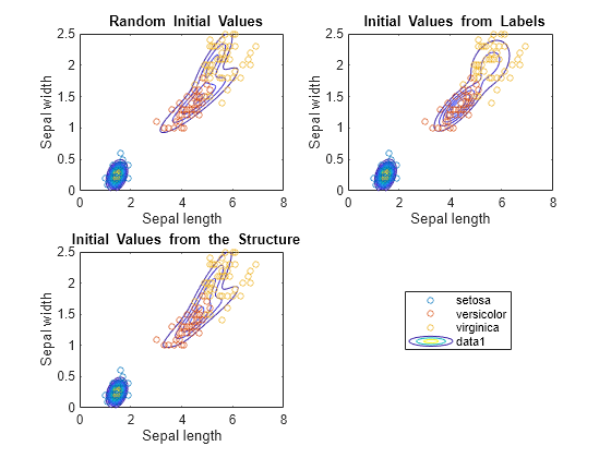
Use gscatter to plot a scatter diagram that distinguishes between the iris species. For each model, plot the fitted Gaussian mixture model contours.
figure
subplot(2,2,1)
h = gscatter(X(:,1),X(:,2),species,[],'o',4);
haxis = gca;
xlim = haxis.XLim;
ylim = haxis.YLim;
d = (max([xlim ylim])-min([xlim ylim]))/1000;
[X1Grid,X2Grid] = meshgrid(xlim(1):d:xlim(2),ylim(1):d:ylim(2));
hold on
contour(X1Grid,X2Grid,reshape(pdf(GMModel1,[X1Grid(:) X2Grid(:)]),...
    size(X1Grid,1),size(X1Grid,2)),20)
uistack(h,'top')
title('{\bf Random Initial Values}');
xlabel('Sepal length');
ylabel('Sepal width');
legend off;
hold off
subplot(2,2,2)
h = gscatter(X(:,1),X(:,2),species,[],'o',4);
hold on
contour(X1Grid,X2Grid,reshape(pdf(GMModel2,[X1Grid(:) X2Grid(:)]),...
    size(X1Grid,1),size(X1Grid,2)),20)
uistack(h,'top')
title('{\bf Initial Values from Labels}');
xlabel('Sepal length');
ylabel('Sepal width');
legend off
hold off
subplot(2,2,3)
h = gscatter(X(:,1),X(:,2),species,[],'o',4);
hold on
contour(X1Grid,X2Grid,reshape(pdf(GMModel3,[X1Grid(:) X2Grid(:)]),...
    size(X1Grid,1),size(X1Grid,2)),20)
uistack(h,'top')
title('{\bf Initial Values from the Structure}');
xlabel('Sepal length');
ylabel('Sepal width');
legend('Location',[0.7,0.25,0.1,0.1]);
hold off

According to the contours, GMModel2 seems to suggest a slight trimodality, while the others suggest bimodal distributions.
Display the estimated component means.
table(GMModel1.mu,GMModel2.mu,GMModel3.mu,'VariableNames',...
    {'Model1','Model2','Model3'})
ans=3×3 table
         Model1               Model2              Model3
    _________________    ________________    ________________

    5.2115     2.0119    4.2857    1.3339    1.4604    0.2429
     1.461    0.24423     1.462     0.246    4.7509    1.4629
    4.6829     1.4429    5.5507    2.0316    5.0158    1.8592
GMModel2 seems to distinguish between the iris species the best.
Input Arguments
Data to which the Gaussian mixture model is fit, specified as a numeric matrix.
The rows of X correspond to observations, and the columns of
X correspond to variables. The number of observations must be
larger than each of the following: the number of variables and the number of
components.
NaNs indicate missing values. The software
removes rows of X containing at least one NaN before
fitting, which decreases the effective sample size.
Data Types: single | double
Number of components to use when fitting Gaussian mixture model,
specified as a positive integer. For example, if you specify k
= 3, then the software fits a Gaussian mixture model with
three distinct means, covariances matrices, and component proportions
to the data (X).
Data Types: single | double
Name-Value Arguments
Specify optional pairs of arguments as
Name1=Value1,...,NameN=ValueN, where Name is
the argument name and Value is the corresponding value.
Name-value arguments must appear after other arguments, but the order of the
pairs does not matter.
Before R2021a, use commas to separate each name and value, and enclose
Name in quotes.
Example: 'RegularizationValue',0.1,'CovarianceType','diagonal' specifies
a regularization parameter value of 0.1 and to fit diagonal covariance
matrices.
Type of covariance matrix to fit to the data, specified as the
comma-separated pair consisting of 'CovarianceType' and
either 'diagonal' or 'full'.
If you set 'diagonal', then the software
fits diagonal covariance matrices. In this case, the software estimates k*d covariance
parameters, where d is the number of columns in X (i.e., d
= size(X,2)).
Otherwise, the software fits full covariance matrices. In this
case, the software estimates k*d*(d+1)/2 covariance
parameters.
Example: 'CovarianceType','diagonal'
Iterative EM algorithm optimization options, specified as the
comma-separated pair consisting of 'Options' and
a statset options structure.
This table describes the available name-value pair arguments.
| Name | Value |
|---|---|
'Display' |
|
'MaxIter' | Positive integer indicating the maximum number of iterations
allowed. The default is 100 |
'TolFun' | Positive scalar indicating the termination tolerance for the
loglikelihood function value. The default is 1e-6. |
Example: 'Options',statset('Display','final','MaxIter',1500,'TolFun',1e-5)
Tolerance for posterior probabilities, specified as the comma-separated pair consisting of
ProbabilityTolerance and a nonnegative scalar value in the range
[0,1e-6].
In each iteration, after the estimation of posterior probabilities, fitgmdist sets
any posterior probability that is not larger than the tolerance value
to zero. Using a nonzero tolerance might speed up fitgmdist.
Example: 'ProbabilityTolerance',0.0000025
Data Types: single | double
Regularization parameter value, specified as the comma-separated
pair consisting of 'RegularizationValue' and a
nonnegative scalar.
Set RegularizationValue to a small positive
scalar to ensure that the estimated covariance matrices are positive
definite.
Example: 'RegularizationValue',0.01
Data Types: single | double
Number of times to repeat the EM algorithm using a new set of
initial values, specified as the comma-separated pair consisting of 'Replicates' and
a positive integer.
If Replicates is greater than 1,
then:
The name-value pair argument
Startmust beplus(the default) orrandSample.GMModelis the fit with the largest loglikelihood.
Example: 'Replicates',10
Data Types: single | double
Flag indicating whether all covariance matrices are identical
(i.e., fit a pooled estimate), specified as the comma-separated pair
consisting of 'SharedCovariance' and either logical
value false or true.
If SharedCovariance is true,
then all k covariance matrices are equal, and the
number of covariance parameters is scaled down by a factor of k.
Initial value setting method, specified as the comma-separated
pair consisting of 'Start' and 'randSample', 'plus',
a vector of integers, or a structure array.
The value of Start determines the initial
values required by the optimization routine for each Gaussian component
parameter — mean, covariance, and mixing proportion. This table
summarizes the available options.
| Value | Description |
|---|---|
'randSample' | The software selects k observations from X at
random as initial component means. The mixing proportions are uniform.
The initial covariance matrices for all components are diagonal, where
the element j on the diagonal is the variance of X(:,j). |
'plus' | The software selects k observations from X using the
k-means++ algorithm. The initial mixing
proportions are uniform. The initial covariance matrices for all components
are diagonal, where the element j on the diagonal is the
variance of X(:,j). |
| Vector of integers | A vector of length n (the number of observations)
containing an initial guess of the component index for each point.
That is, each element is an integer from 1 to k,
which corresponds to a component. The software collects all observations
corresponding to the same component, computes means, covariances,
and mixing proportions for each, and sets the initial values to these
statistics. |
| Structure array |
Suppose that there are
|
Example: 'Start',ones(n,1)
Data Types: single | double | char | string | struct
Output Arguments
Fitted Gaussian mixture model, returned as a gmdistribution model.
Access properties of GMModel using dot notation.
For example, display the AIC by entering GMModel.AIC.
Tips
fitgmdist might:
Converge to a solution where one or more of the components has an ill-conditioned or singular covariance matrix.
The following issues might result in an ill-conditioned covariance matrix:
The number of dimensions of your data is relatively high and there are not enough observations.
Some of the predictors (variables) of your data are highly correlated.
Some or all the features are discrete.
You tried to fit the data to too many components.
In general, you can avoid getting ill-conditioned covariance matrices by using one of the following precautions:
Preprocess your data to remove correlated features.
Set
'SharedCovariance'totrueto use an equal covariance matrix for every component.Set
'CovarianceType'to'diagonal'.Use
'RegularizationValue'to add a very small positive number to the diagonal of every covariance matrix.Try another set of initial values.
Pass through an intermediate step where one or more of the components has an ill-conditioned covariance matrix. Try another set of initial values to avoid this issue without altering your data or model.
Algorithms
The software optimizes the Gaussian mixture model likelihood using the iterative Expectation-Maximization (EM) algorithm.
fitgmdist fits GMMs to data using the iterative Expectation-Maximization (EM) algorithm. Using initial values for component means, covariance matrices, and mixing proportions, the EM algorithm proceeds using these steps.
For each observation, the algorithm computes posterior probabilities of component memberships. You can think of the result as an n-by-k matrix, where element (i,j) contains the posterior probability that observation i is from component j. This is the E-step of the EM algorithm.
Using the component-membership posterior probabilities as weights, the algorithm estimates the component means, covariance matrices, and mixing proportions by applying maximum likelihood. This is the M-step of the EM algorithm.
The algorithm iterates over these steps until convergence. The likelihood surface is complex, and the algorithm might converge to a local optimum. Also, the resulting local optimum might depend on the initial conditions. fitgmdist has several options for choosing initial conditions, including random component assignments for the observations and the k-means ++ algorithm.
The k-means++ algorithm
uses an heuristic to find centroid seeds for k-means
clustering. fitgmdist can apply the same principle
to initialize the EM algorithm by using the k-means++ algorithm to
select the initial parameter values for a fitted Gaussian mixture
model.
The k-means++ algorithm assumes the number of clusters is k and chooses the initial parameter values as follows.
Select the component mixture probability to be the uniform probability , where i = 1, ..., k.
Select the covariance matrices to be diagonal and identical, where and .
Select the first initial component center μ1 uniformly from all data points in X.
To choose center j:
Compute the Mahalanobis distances from each observation to each centroid, and assign each observation to its closest centroid.
For m = 1,...,n and p = 1,...,j – 1, select centroid j at random from X with probability
where is the distance between observation m and μp, and Mp is the set of all observations closest to centroid μp and xm belongs to Mp.
That is, select each subsequent center with a probability proportional to the distance from itself to the closest center that you already chose.
Repeat step 4 until k centroids are chosen.
References
[1] McLachlan, G., and D. Peel. Finite Mixture Models. Hoboken, NJ: John Wiley & Sons, Inc., 2000.
Version History
Introduced in R2014a
MATLAB Command
You clicked a link that corresponds to this MATLAB command:
Run the command by entering it in the MATLAB Command Window. Web browsers do not support MATLAB commands.
Website auswählen
Wählen Sie eine Website aus, um übersetzte Inhalte (sofern verfügbar) sowie lokale Veranstaltungen und Angebote anzuzeigen. Auf der Grundlage Ihres Standorts empfehlen wir Ihnen die folgende Auswahl: .
Sie können auch eine Website aus der folgenden Liste auswählen:
So erhalten Sie die bestmögliche Leistung auf der Website
Wählen Sie für die bestmögliche Website-Leistung die Website für China (auf Chinesisch oder Englisch). Andere landesspezifische Websites von MathWorks sind für Besuche von Ihrem Standort aus nicht optimiert.
Amerika
- América Latina (Español)
- Canada (English)
- United States (English)
Europa
- Belgium (English)
- Denmark (English)
- Deutschland (Deutsch)
- España (Español)
- Finland (English)
- France (Français)
- Ireland (English)
- Italia (Italiano)
- Luxembourg (English)
- Netherlands (English)
- Norway (English)
- Österreich (Deutsch)
- Portugal (English)
- Sweden (English)
- Switzerland
- United Kingdom (English)