Multiloop Control Design for Buck Converter
This example shows how to tune the gains of a discrete PID controller in a cascade control configuration using systune.
This example is based on the article Cascade Digital PID Control Design for Power Electronic Converters. The article describes the workflow to tune the inner-loop current control and outer-loop voltage control one loop at a time, whereas this example shows how to tune both loops at the same time.
In this example, you:
Conduct frequency response estimation (FRE) of the buck converter plant model.
Estimate a parametric LTI model from the FRE result.
Construct a multiloop feedback control system using LTI models.
Define tuning goals in the frequency domain and tune the controllers using
systune.Verify the performance of the tuned controllers.
Conduct Frequency Response Estimation
This example uses a buck converter modeled using Simscape™ Electrical™ components to provide voltage regulation from 48 V to 12 V. The model uses cascade control architecture so that the inner loop regulates the inductor current and the outer loop regulates the output voltage. The output of the outer voltage loop provides the current reference signal to the inner current loop, which, in turn, provides the duty cycle signal to the PWM Generator block. The controller architecture includes manual switches to make the converter operate in one of three configurations: open-loop (PWM Generator block with a constant duty cycle), inner current-loop, and outer voltage loop.
Open the buck converter plant model.
mdl = "scdCurrentControlBuckConverter";
open_system(mdl)
Specify Linear Analysis Points for Frequency Response Estimation
To collect frequency response data, you must first specify the portion of model to estimate. You can configure the linear analysis points that specify the inputs and outputs of the model for estimation using linio. Alternatively, you can interactively specify the linear analysis points using the Linearization Manager app. Here, use linio to assign the input perturbation analysis point to the Duty Cycle block and the output measurement analysis points to the Current ADC and Voltage ADC blocks, which are the Rate Transition blocks after the inductor current measurement and output voltage measurement Probe blocks, respectively.
io(1) = linio("scdCurrentControlBuckConverter/Duty Cycle",1,"input");
io(2) = linio("scdCurrentControlBuckConverter/Current ADC",1,"output");
io(3) = linio("scdCurrentControlBuckConverter/Voltage ADC",1,"output");
Find Snapshot-Based Model Operating Point and Initialize Model
To obtain a frequency response that accurately captures system dynamics, you must perform the estimation at a steady-state operating point.
Simulate the model to determine the time the model takes to reach steady state.
sim(mdl,"StopTime","0.008");
open_system(mdl + "/Scope")
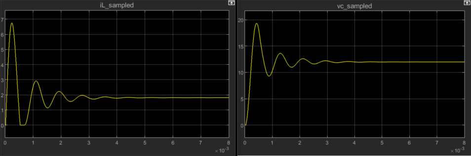
open_system(mdl + "/Scope2")
Close the scopes to improve simulation time during estimation.
close_system(mdl + "/Scope")
close_system(mdl + "/Scope2")
Initial simulation results show that the buck converter model reaches steady-state operation after around 0.007 seconds. Take a simulation snapshot at 0.007 seconds to find the steady-state operating point.
opini = findop(mdl,0.007);
Initialize the model using this operating point object.
set_param(mdl,"LoadInitialState","on","InitialState","getstatestruct(opini)");
op = operpoint(mdl);
Create Perturbation Signal for Experiment and Compute Non-Parametric Frequency Response
Define a PRBS perturbation signal with the following parameters.
Signal order — 11
Number of periods — 1
Perturbation amplitude — 0.05
Sample time — seconds
in_PRBS = frest.PRBS(Order=11,NumPeriods=1,Amplitude=0.05,Ts=1e-5);
Before you conduct the frequency response estimation experiment, identify the time-varying sources so that these sources are deterministic during the experiment.
srcblks = frest.findSources(mdl,io);
opts = frestimateOptions;
opts.BlocksToHoldConstant = srcblks;
You can now conduct the frequency response estimation experiment. During the experiment, the software simulates the model, injects the PRBS signal at the specified input, and measures the response at the specified output. The result is a frequency-response data model (frd) object. This is a non-parametric model that is a description of the system as discrete frequency points.
estsys_PRBS = frestimate(mdl,io,op,in_PRBS,opts);
Frequency response estimation with PRBS input signal produces results with many frequency points. Use interp (System Identification Toolbox) to extract an interpolated result from the estimated frequency response model across 50 frequency points from 700 rad/s to 300,000 rad/s.
wmin = 700;
wmax = 3e5;
Nfreq = 50;
w = logspace(log10(wmin+10),log10(wmax),Nfreq);
estsys_PRBS_thinned = interp(estsys_PRBS, w);
Compare the FRE result before and after thinning.
figure
bodeplot(estsys_PRBS,estsys_PRBS_thinned);
legend("Raw FRE result","Thinned FRE result");

The frequency points match very well. You can now estimate a parametric model from the thinned result.
Estimate Parametric LTI Model from FRE Results
Estimate a state-space parametric model of the buck converter with one input (duty cycle) and two outputs (inductor current and output voltage). As the shape of the estimated frequency response in the Bode plot resembles a third-order model, estimate a third-order state-space model using ssest.
optssest = ssestOptions(SearchMethod="lm");
optssest.Regularization.Lambda = 1e-8;
sys_systune = ssest(estsys_PRBS_thinned,3,"Ts",Ts_ctrl,optssest);
Compare the parametric estimation result with the thinned FRE result.
figure
bp = bodeplot(estsys_PRBS_thinned,sys_systune);
bp.PhaseMatchingEnabled = "on";
legend("FRE result","ssest result");

You can see that the estimated parametric model is satisfactory.
Construct Feedback Control System for Tuning
To model a feedback control system for tuning, first define the discrete-time PI controllers as tunable elements.
Ci = tunablePID("Ci","PI",Ts_ctrl);
Ci.IFormula = "Trapezoidal";
Ci.u = "Ie";
Ci.y = "Duty Cycle";

Cv = tunablePID("Cv","PI",Ts_ctrl);
Cv.IFormula = "Trapezoidal";
Cv.u = "Ve";
Cv.y = "Iref";
To improve the convergence time, provide initial values for the outer-loop controller.
Cv.Kp.Value = 1;
Cv.Ki.Value = 200;
Then, construct a multiloop control system as shown.
sum_i = sumblk("Ie = Iref-iL_sampled");
sum_v = sumblk("Ve = Vref-vc_sampled");

input = {"Vref"};
output = {"iL_sampled","vc_sampled"};
APs = {"Iref","Duty Cycle","iL_sampled","vc_sampled"};

ST0 = connect(sys_systune,Ci,Cv,sum_i,sum_v,input,output,APs);
Define Frequency-Domain Tuning Goals
Define tuning goals for inner and outer loops using target bandwidths and stability margins.
Use
TuningGoal.LoopShapeto specify the target bandwidth.Use
TuningGoal.Marginsto specify phase and gain margins in a frequency range. While you can clearly define target phase margins, specify a small value of 3 dB for the gain margins for stability. The tuning result usually achieves a higher gain margin. For this goal, also define a frequency focus band so thatsystuneenforces margins only over the interested frequency range.
Additionally, specify the outer loop as open while evaluating the inner-loop tuning goals.
LS1 = TuningGoal.LoopShape("iL_sampled",30000);
LS1.Openings = {"vc_sampled"};
LS2 = TuningGoal.LoopShape("vc_sampled",3000);
MG1 = TuningGoal.Margins("iL_sampled",3,60);
MG1.Openings = {"vc_sampled"};
MG1.Focus = [30000 300000];
MG2 = TuningGoal.Margins("vc_sampled",3,60);
MG2.Focus = [3000 30000];
Tune Controllers and Extract Tuning Results
Start tuning with systune, using the following settings to help optimization achieve desirable results. To satisfy the performance requirements, systune enforces all tuning goals as hard goals.
Create a systuneOptions object and adjust the values for the minimum decay rate and maximum spectral radius to suit tuning for high bandwidth loop shapes. Also, reduce the relative tolerance criteria for termination.
opt = systuneOptions(SoftTol=1e-10,MinDecay=1e-10,MaxRadius=1e10);
rng(1)
[ST1,fSoft,fHard] = systune(ST0,[],[LS1,LS2,MG1,MG2],opt);
Final: Soft = -Inf, Hard = 1.6989, Iterations = 78
Plot the performance of the tuned system against the tuning goals.
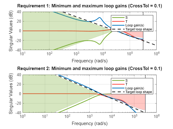
figure
viewGoal([LS1,LS2],ST1)
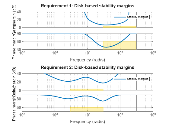
figure
viewGoal([MG1,MG2],ST1)
For the inner loop, the tuned result achieves a bandwidth slightly lower than the specified target bandwidth and the phase margin is lower than the specified target phase margin in some frequencies. Even though the tuning goals are not completely satisfied, the tuning results are sufficient for the stable operation of the tuned model.
Get the controller gains from tunable blocks and save to workspace.
Cv = getBlockValue(ST1,'Cv');
Ci = getBlockValue(ST1,'Ci');
CurrentControlP = Ci.Kp
CurrentControlP =
0.1392
CurrentControlI = Ci.Ki
CurrentControlI =
1.8703e+03
VoltageControlP = Cv.Kp
VoltageControlP =
0.0186
VoltageControlI = Cv.Ki
VoltageControlI =
306.9463
Verify Control Design Result Performance
Examine the tuned controller performance with load and input voltage disturbances.
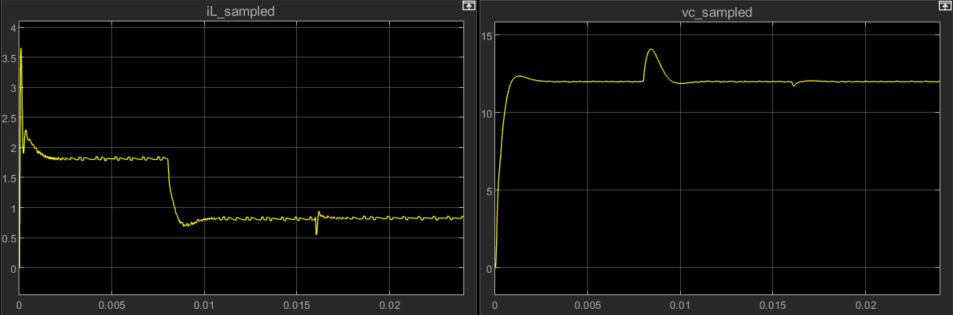
The load disturbance is applied at 0.008 seconds, which increases the load resistance from 6 ohms to 12 ohms.
The input voltage disturbance is applied at 0.016 seconds, which decreases the input voltage from 48 V to 40 V.
Set the PI controller gains to the tuned values.
set_param("scdCurrentControlBuckConverter/Discrete PID Controller","P","CurrentControlP");
set_param("scdCurrentControlBuckConverter/Discrete PID Controller","I","CurrentControlI");
set_param("scdCurrentControlBuckConverter/Discrete PID Controller1","P","VoltageControlP");
set_param("scdCurrentControlBuckConverter/Discrete PID Controller1","I","VoltageControlI");
Toggle the manual switches to close both the inner and outer loops and simulate the model with the regulated voltage and current.
set_param("scdCurrentControlBuckConverter/Manual Switch","sw","0");
set_param("scdCurrentControlBuckConverter/Manual Switch1","sw","0");
Simulate the model with the tuned gains.
set_param(mdl,"LoadInitialState","off");
sim(mdl)
open_system(mdl + "/Scope")
open_system(mdl + "/Scope2")
The tuned controllers track the voltage reference and reject disturbances well. To fine tune the result, you can update the tuning goals in the Define Frequency-Domain Tuning Goals section of this example. For a faster response, you can increase the target bandwidth in the loop shape tuning goal. For improved transient behavior, you can increase the target phase margin in the margins tuning goal.
See Also
systune | ssest (System Identification Toolbox) | frestimate | connect