Model Linearizer

Linearize Simulink models

Description

Model Linearizer lets you perform linear analysis of nonlinear Simulink^® models.

Using this app, you can:

• Interactively linearize models at different operating points

• Interactively obtain operating points by trimming or simulating models

• Perform exact linearization of nonlinear models

• Perform frequency response estimation of nonlinear models

• Batch linearize models for varying parameter values

• Generate MATLAB^® code for performing linearization tasks

• Generate MATLAB code for computing operating points

Limitations

• Linearization is not supported for model hierarchies that contain referenced models configured to use a local solver.

• Linearization is not supported for Simscape™ networks configured to use a local solver.

Open the Model Linearizer App

• Simulink Toolstrip: On the Apps tab, under Control Systems, click Model Linearizer.

• Simulink Toolstrip: On the Apps tab, under Control Systems, click Frequency Response Estimator.

• Simulink Toolstrip: On the Linearization tab, click Model Linearizer.

• Simulink Toolstrip: On the Linearization tab, click Frequency Response Estimator.

• Simulink Toolstrip: On the Linearization tab, click Linearize Block.

Examples

Export Linearization or Estimation Results

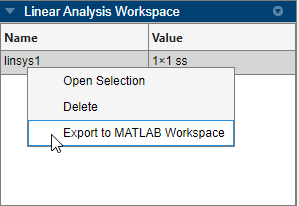
To export your linearization or estimation result to the MATLAB workspace, on the Plots and Results tab, click Export Result.

Alternatively, to export a model, in the data browser, in the Linear Analysis Workspace right-click the model and select Export to MATLAB Workspace.

Export Batch Linearization Results as LPV or LTV Model

You can export your batch linearization results as either a linear parameter-varying (LPV) or linear time-varying (LTV) model.

1. Configure a batch linearization by specifying either of these settings for your linearization:

   • Parameter grid (for LPV models) — For more information on specifying a parameter grid, see Batch Linearize Model for Parameter Value Variations Using Model Linearizer.

   • Snapshot times (for LTV models) — In this case, you must specify a vector of snapshot times using Operating Point > Linearize At and not an array of operating points computed from snapshot times.

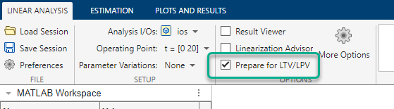
2. On the Linear Analysis tab, select Prepare for LTV/LPV.

   

3. Linearize the model.

4. On the Plots and Results tab, click Export as LTV/LPV.

5. In the Export LTV/LPV Model dialog box, select a linearization result in the table.

   

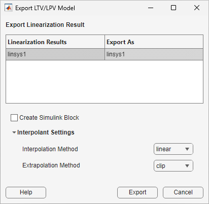
6. In the Export As column, specify a name for the variable in the MATLAB workspace.

7. To create a model that contains an LPV System or LTV System block that uses the exported model, select Create Simulink Block.

8. Under Interpolation Method, select one of these methods for interpolating between linear models.

   • linear

   • nearest

   • next

   • previous

   • pchip

   • cubic

   • spline

   • makima

   When creating a Simulink model for your linearization result, you can specify the interpolation method as linear, nearest, or flat.

9. Under Extrapolation Method, select one of these methods for extrapolating beyond the available linear models. For more information on interpolation and extrapolation methods, see griddedInterpolant and scatteredInterpolant.

   • clip

   • linear

   • nearest

   • next

   • previous

   • pchip

   • cubic

   • spline

   • makima

   When creating a Simulink model for your linearization result, you can specify the interpolation method as clip or linear.

10. Click Export.

Related Examples

• Linearize Simulink Model at Model Operating Point
• Linearize at Trimmed Operating Point
• Linearize at Simulation Snapshot
• Estimate Frequency Response Using Model Linearizer
• Specify Portion of Model to Linearize in Model Linearizer
• Analyze Results Using Model Linearizer Response Plots
• View Linearized Model Equations Using Model Linearizer
• Batch Linearize Model for Parameter Value Variations Using Model Linearizer

Parameters

Linear Analysis Tab

Analysis I/Os — Linearization inputs, outputs, and loop openings

Model I/Os (default) | linearization I/O set

Linearization inputs, outputs, and loop openings. The currently active I/O set is displayed. To change the I/O set, select one of the following:

• Model I/Os — Use the inputs, outputs, and loop openings specified in the Simulink model. For more information on specifying analysis points in your model, see Specify Portion of Model to Linearize in Simulink Model.

• Root Level Inports and Outports — Use the root level inputs and outputs of the Simulink model.

• Linearize the Currently Selected Block — Use the input and output ports of the currently selected block in the Simulink model.

• Create New Linearization I/Os — Specify inputs, outputs, and loop openings. For more information, see Specify Portion of Model to Linearize in Model Linearizer.

• Existing I/Os — Select a previously created I/O set.

• View/Edit — View or edit the currently selected operating point. For more information, see Edit Analysis Points.

Operating Point — Linearization operating point

Model Initial Condition (default) | operating point

Linearization operating point. The current operating point is displayed. To change the operating point, select one of the following:

• Model Initial Condition — Use the initial conditions defined in the Simulink.

• Linearize At — Simulate the model using the model initial conditions, and use the simulation snapshot at the specified time as the operating point. For more information, see Linearize at Simulation Snapshot.

• Linearize at Multiple Points — Select multiple previously created operating points.

• Existing Operating points — Select a previously created operating point.

• Trim Model — Compute a steady-state operating point. For more information, see Compute Steady-State Operating Points.

• Take Simulation Snapshot — Simulate the model using the model initial conditions, and compute an operating point at the specified simulation snapshot times. For more information, see Find Operating Points at Simulation Snapshots.

• View/Edit — View or edit the currently selected operating point.

Parameter Variations — Parameters to vary for batch linearization

None (default) | parameters to vary

To vary parameters for batch linearization, in the drop-down list, click Select parameters to vary. On the Parameter Variations tab, specify the parameters to vary.

Parameter variation is not supported when linearizing your model using numerical perturbation.

For more information, see Specify Parameter Samples for Batch Linearization.

Result Viewer — Open linearization result viewer

off (default) | on

Select to display result details after linearization. For more information, see View Linearized Model Equations Using Model Linearizer.

Linearization Advisor — Collect diagnostic information and open Linearization Advisor

off (default) | on

Select to collect diagnostic information during linearization and open an Advisor tab for interactive troubleshooting of linearization problems. For more information, see Troubleshoot Linearization Results in Model Linearizer.

Note

Model Linearizer only collects diagnostic information when you select Linearization Advisor before linearizing the model.

Prepare for LTV/LPV — Configure linearization options for LTV/LPV generation

off (default) | on

To generate a linear time-varying (LTV) or linear parameter-varying (LPV) model from your batch linearization results, you must select Prepare for LTV/LPV before linearizing your model.

When you select Prepare for LTV/LPV, Model Linearizer sets the following linearization options.

• Sets the Block reduction scope option to Consistent across models, which ensures that all linearized models in the batch linearization results have a consistent state definition. This setting means that the software removes only the states and delays that do not contribute to the input-output map for all models in the array of linearized models.

• Selects the Store offsets with linear model option. The software stores any operating point offsets values in the resulting linearized model and exports the offset values with the LPV/LTV model.

If you manually specify these linearization options instead of selecting Prepare for LTV/LPV, you can still export your linearization results as an LTV or LPV model.

Dependencies

This option is available if you define a batch linearization by specifying either a parameter grid (LPV) or a vector of snap shot times (LTV).

Estimation Tab

Input Signal — Estimation input signal

Sinestream | Fixed Sample Time Sinestream | Chirp | Random | PRBS Pseudorandom Binary Sequence

Estimation input signal. The current input signal is displayed. To change the input signal, select one of the following:

• Sinestream — Create an input signal that consists of adjacent sine waves of varying frequencies. For more information, see Sinestream Input Signals.

• Fixed Sample Time Sinestream — Create a discrete-time sinestream input with a specified sample time.

• Chirp — Create a swept-frequency cosine input signal. For more information, see Chirp Input Signals.

• Random — Create a random input signal.

• PRBS Pseudorandom Binary Sequence — Create a pseudorandom binary sequence (PRBS) input signal. For more information, see PRBS Input Signals.

Analysis I/Os — Linearization inputs, outputs, and loop openings

Model I/Os (default) | linearization I/O set

Linearization inputs, outputs, and loop openings. The currently active I/O set is displayed. To change the I/O set, select one of the following:

• Model I/Os — Use the inputs, outputs, and loop openings specified in the Simulink model. For more information on specifying analysis points in your model, see Specify Portion of Model to Linearize in Simulink Model.

• Root Level Inports and Outports — Use the root level inputs and outputs of the Simulink model.

• Linearize the Currently Selected Block — Use the input and output ports of the currently selected block in the Simulink model.

• Create New Linearization I/Os — Specify inputs, outputs, and loop openings. For more information, see Specify Portion of Model to Linearize in Model Linearizer.

• Existing I/Os — Select a previously created I/O set.

• View/Edit — View or edit the currently selected operating point. For more information, see Edit Analysis Points.

Operating Point — Linearization operating point

Model Initial Condition (default) | operating point

Linearization operating point. The current operating point is displayed. To change the operating point, select one of the following:

• Model Initial Condition — Use the initial conditions defined in the Simulink.

• Linearize At — Simulate the model using the model initial conditions, and use the simulation snapshot at the specified time as the operating point. For more information, see Linearize at Simulation Snapshot.

• Linearize at Multiple Points — Select multiple previously created operating points.

• Existing Operating points — Select a previously created operating point.

• Trim Model — Compute a steady-state operating point. For more information, see Compute Steady-State Operating Points.

• Take Simulation Snapshot — Simulate the model using the model initial conditions, and compute an operating point at the specified simulation snapshot times. For more information, see Find Operating Points at Simulation Snapshots.

• View/Edit — View or edit the currently selected operating point.

Result Viewer — Open estimation result viewer

off (default) | on

Select to display result details about the estimation configuration and input signal used for estimation.

Diagnostic Viewer — Collect diagnostic information and open diagnostic viewer

off (default) | on

Select to collect diagnostic information that displays after estimation. You can use the diagnostic information to analyze the estimation result and troubleshoot estimation problems. For more information, see Analyze Estimated Frequency Response.

Note

Model Linearizer only collects diagnostic information when Diagnostic Viewer is selected before performing an estimation task.

Version History

Introduced in R2011b

R2026a: Obtain LPV or LTV model from batch linearization result

You can now obtain a linear parameter-varying (LPV) and linear time-varying (LTV) models from batch linearization results in the Model Linearizer app. For more information, see Export Batch Linearization Results as LPV or LTV Model.

R2023b: Simulink Online support

Starting in R2023b, Model Linearizer is supported in Simulink Online™.

R2021b: Linearize Simulink model to sparse state-space model

Using Model Linearizer, you can obtain a sparse linear model from a Simulink model that contains a Sparse Second Order or Descriptor State-Space block. For more information, see Linearize Sparse Models.

R2021a: Automatically determine PRBS estimation input signal parameters

When creating PRBS input signals for estimating frequency responses in Model Linearizer, you can now automatically determine the signal parameters Number of periods and Signal order based on a frequency range.

R2021a: Result thinning for frequency response estimation

When you have an estimated frequency response result with a large number of frequency points, you can use result thinning in Model Linearizer to extract interpolated frequency response data from an estimated frequency response model across a specified frequency range and number of frequency points. For more information, see Analyze Estimated Frequency Response.

R2020a: Linear Analysis Tool is now Model Linearizer

The Linear Analysis Tool is now the Model Linearizer app. The features of the app remain the same, only the name has changed.

R2020a: PRBS input signals for frequency response estimation

You can now estimate the frequency response of your Simulink model using pseudorandom binary sequence (PRBS) input signals. For more information, see PRBS Input Signals.