generate
Generate scenarios from SimBiology.Scenarios object and return
table
Syntax
Description
scenariosTable = generate(sObj)SimBiology.Scenarios object
sObj and returns a table, where each row represents a scenario and
each column represents an entry.
scenariosTable = generate(sObj,n)nth row
(scenario) of the scenarios table.
scenariosTable = generate(___,'StandardizedOutput',tf)
Examples
Load the model of glucose-insulin response. For details about the model, see the Background section in Simulate the Glucose-Insulin Response.
sbioloadproject('insulindemo','m1');
The model contains different parameter values and initial conditions that represents different insulin impairments (such as Type 2 diabetes, low insulin sensitivity, and so on) stored in five variants.
variants = getvariant(m1)
variants =
   SimBiology Variant Array

   Index:  Name:             Active:
   1       Type 2 diabetic   false
   2       Low insulin se... false
   3       High beta cell... false
   4       Low beta cell ... false
   5       High insulin s... false
Suppress an informational warning that is issued during simulations.
warnSettings = warning('off','SimBiology:DimAnalysisNotDone_MatlabFcn_Dimensionless');
Select a dose that represents a single meal of 78 grams of glucose.
singleMeal = sbioselect(m1,'Name','Single Meal');
Create a Scenarios object to represent different initial conditions combined with the dose. That is, create a scenario object where each variant is paired (or combined) with the dose, for a total of five simulation scenarios.
sObj = SimBiology.Scenarios;
add(sObj,'cartesian','variants',variants);
add(sObj,'cartesian','dose',singleMeal)
ans =
  Scenarios (5 scenarios)

                   Name            Content          Number
                 ________    ___________________    ______

    Entry 1      variants    SimBiology variants      5
    x Entry 2    dose        SimBiology dose          1

  See also Expression property.
sObj contains two entries. Use the generate function to combine the entries and generate five scenarios. The function returns a scenarios table, where each row represents a scenario and each column represents an entry of the Scenarios object.
scenariosTbl = generate(sObj)
scenariosTbl=5×2 table
           variants                     dose
    ______________________    _________________________

    1×1 SimBiology.Variant    1×1 SimBiology.RepeatDose
    1×1 SimBiology.Variant    1×1 SimBiology.RepeatDose
    1×1 SimBiology.Variant    1×1 SimBiology.RepeatDose
    1×1 SimBiology.Variant    1×1 SimBiology.RepeatDose
    1×1 SimBiology.Variant    1×1 SimBiology.RepeatDose
Change the entry name of the first entry.
rename(sObj,1,'Insulin Impairements')ans =
Scenarios (5 scenarios)
Name Content Number
____________________ ___________________ ______
Entry 1 Insulin Impairements SimBiology variants 5
x Entry 2 dose SimBiology dose 1
See also Expression property.
Create a SimFunction object to simulate the generated scenarios. Use the Scenarios object as the input and specify the plasma glucose and insulin concentrations as responses (outputs of the function to be plotted). Specify [] for the dose input argument since the Scenarios object already has the dosing information.
f = createSimFunction(m1,sObj,{'[Plasma Glu Conc]','[Plasma Ins Conc]'},[])f =
SimFunction
Parameters:
Name Value Type Units
___________________________ ______ _____________ ___________________________________________
{'[Plasma Volume (Glu)]' } 1.88 {'parameter'} {'deciliter' }
{'k1' } 0.065 {'parameter'} {'1/minute' }
{'k2' } 0.079 {'parameter'} {'1/minute' }
{'[Plasma Volume (Ins)]' } 0.05 {'parameter'} {'liter' }
{'m1' } 0.19 {'parameter'} {'1/minute' }
{'m2' } 0.484 {'parameter'} {'1/minute' }
{'m4' } 0.1936 {'parameter'} {'1/minute' }
{'m5' } 0.0304 {'parameter'} {'minute/picomole' }
{'m6' } 0.6469 {'parameter'} {'dimensionless' }
{'[Hepatic Extraction]' } 0.6 {'parameter'} {'dimensionless' }
{'kmax' } 0.0558 {'parameter'} {'1/minute' }
{'kmin' } 0.008 {'parameter'} {'1/minute' }
{'kabs' } 0.0568 {'parameter'} {'1/minute' }
{'kgri' } 0 {'parameter'} {'1/minute' }
{'f' } 0.9 {'parameter'} {'dimensionless' }
{'a' } 0 {'parameter'} {'1/milligram' }
{'b' } 0.82 {'parameter'} {'dimensionless' }
{'c' } 0 {'parameter'} {'1/milligram' }
{'d' } 0.01 {'parameter'} {'dimensionless' }
{'kp1' } 2.7 {'parameter'} {'milligram/minute' }
{'kp2' } 0.0021 {'parameter'} {'1/minute' }
{'kp3' } 0.009 {'parameter'} {'(milligram/minute)/(picomole/liter)' }
{'kp4' } 0.0618 {'parameter'} {'(milligram/minute)/picomole' }
{'ki' } 0.0079 {'parameter'} {'1/minute' }
{'[Ins Ind Glu Util]' } 1 {'parameter'} {'milligram/minute' }
{'Vm0' } 2.5129 {'parameter'} {'milligram/minute' }
{'Vmx' } 0.047 {'parameter'} {'(milligram/minute)/(picomole/liter)' }
{'Km' } 225.59 {'parameter'} {'milligram' }
{'p2U' } 0.0331 {'parameter'} {'1/minute' }
{'K' } 2.28 {'parameter'} {'picomole/(milligram/deciliter)' }
{'alpha' } 0.05 {'parameter'} {'1/minute' }
{'beta' } 0.11 {'parameter'} {'(picomole/minute)/(milligram/deciliter)'}
{'gamma' } 0.5 {'parameter'} {'1/minute' }
{'ke1' } 0.0005 {'parameter'} {'1/minute' }
{'ke2' } 339 {'parameter'} {'milligram' }
{'[Basal Plasma Glu Conc]'} 91.76 {'parameter'} {'milligram/deciliter' }
{'[Basal Plasma Ins Conc]'} 25.49 {'parameter'} {'picomole/liter' }
Observables:
Name Type Units
_____________________ ___________ _______________________
{'[Plasma Glu Conc]'} {'species'} {'milligram/deciliter'}
{'[Plasma Ins Conc]'} {'species'} {'picomole/liter' }
Dosed:
TargetName TargetDimension
__________ _____________________
{'Dose'} {'Mass (e.g., gram)'}
TimeUnits: hour
Simulate the model for 24 hours and plot the simulation data. The data contains five runs, where each run represents a scenario in the Scenarios object.
sd = f(sObj,24);
sbioplot(sd)
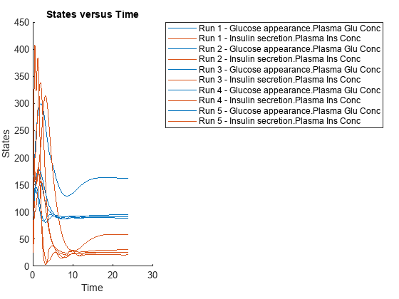
ans =
  Axes (SbioPlot) with properties:

             XLim: [0 30]
             YLim: [0 450]
           XScale: 'linear'
           YScale: 'linear'
    GridLineStyle: '-'
         Position: [0.0878 0.1127 0.2999 0.8123]
            Units: 'normalized'

  Show all properties
If you have Statistics and Machine Learning Toolbox™, you can also draw sample values for model quantities from various probability distributions. For instance, suppose that the parameters Vmx and kp3, which are known for the low and high insulin sensitivity, follow the lognormal distribution. You can generate sample values for these parameters from such a distribution, and perform a scan to explore model behavior.
Define the lognormal probability distribution object for Vmx.
pd_Vmx = makedist('lognormal')pd_Vmx =
LognormalDistribution
Lognormal distribution
mu = 0
sigma = 1
By definition, the parameter mu is the mean of logarithmic values. To vary the parameter value around the base (model) value of the parameter, set mu to log(model_value). Set the standard deviation (sigma) to 0.2. For a small sigma value, the mean of a lognormal distribution is approximately equal to log(model_value). For details, see Lognormal Distribution (Statistics and Machine Learning Toolbox).
Vmx = sbioselect(m1,'Name','Vmx');
pd_Vmx.mu = log(Vmx.Value);
pd_Vmx.sigma = 0.2
pd_Vmx =
  LognormalDistribution

  Lognormal distribution
       mu = -3.05761
    sigma =      0.2
Similarly define the probability distribution for kp3.
pd_kp3 = makedist('lognormal');
kp3 = sbioselect(m1,'Name','kp3');
pd_kp3.mu = log(kp3.Value);
pd_kp3.sigma = 0.2
pd_kp3 =
  LognormalDistribution

  Lognormal distribution
       mu = -4.71053
    sigma =      0.2
Now define a joint probability distribution to draw sample values for Vmx and kp3, with a rank correlation to specify some correlation between these two parameters. Note that this correlation assumption is for the illustration purposes of this example only and may not be biologically relevant.
First remove the variants entry (entry 1) from sObj.
remove(sObj,1)
ans =
  Scenarios (1 scenarios)

               Name        Content        Number
               ____    _______________    ______

    Entry 1    dose    SimBiology dose      1

  See also Expression property.
Add an entry that defines the joint probability distribution with a rank correlation matrix.
add(sObj,'cartesian',["Vmx","kp3"],[pd_Vmx, pd_kp3],'RankCorrelation',[1,0.5;0.5,1])
ans =
  Scenarios (2 scenarios)

                    Name           Content              Number
                    ____    ______________________    ___________

    Entry 1         dose    SimBiology dose           1
    x (Entry 2.1    Vmx     Lognormal distribution    2 (default)
    + Entry 2.2)    kp3     Lognormal distribution    2 (default)

  See also Expression property.
By default, the number of samples to draw from the joint distribution is set to 2. Increase the number of samples.
updateEntry(sObj,2,'Number',50)ans =
Scenarios (50 scenarios)
Name Content Number
____ ______________________ ______
Entry 1 dose SimBiology dose 1
x (Entry 2.1 Vmx Lognormal distribution 50
+ Entry 2.2) kp3 Lognormal distribution 50
See also Expression property.
Verify that the Scenarios object can be simulated with the model. The verify function throws an error if any entry does not resolve uniquely to an object in the model or the entry contents have inconsistent lengths (sample sizes). The function throws a warning if multiple entries resolve to the same object in the model.
verify(sObj,m1)
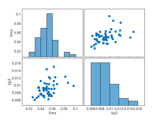
Generate the simulation scenarios. Plot the sample values using plotmatrix. You can see the value of Vmx is varied around its model value 0.047 and that of kp3 around 0.009.
sTbl = generate(sObj); [s,ax,bigax,h,hax] = plotmatrix([sTbl.Vmx,sTbl.kp3]); ax(1,1).YLabel.String = "Vmx"; ax(2,1).YLabel.String = "kp3"; ax(2,1).XLabel.String = "Vmx"; ax(2,2).XLabel.String = "kp3";
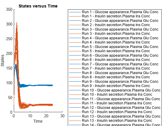
Simulate the scenarios using the same SimFunction you created previously. You do not need to create a new SimFunction object even though the Scenarios object has been updated.
sd2 = f(sObj,24); sbioplot(sd2);
By default, SimBiology uses the random sampling method. You can change it to the Latin hypercube sampling (or sobol or halton) for a more systematic space-filling approach.
entry2struct = getEntry(sObj,2)
entry2struct = struct with fields:
Name: {'Vmx' 'kp3'}
Content: [2×1 prob.LognormalDistribution]
Number: 50
RankCorrelation: [2×2 double]
Covariance: []
SamplingMethod: 'random'
SamplingOptions: [0×0 struct]
entry2struct.SamplingMethod = 'lhs'entry2struct = struct with fields:
Name: {'Vmx' 'kp3'}
Content: [2×1 prob.LognormalDistribution]
Number: 50
RankCorrelation: [2×2 double]
Covariance: []
SamplingMethod: 'lhs'
SamplingOptions: [0×0 struct]
You can now use the updated structure to modify entry 2.
updateEntry(sObj,2,entry2struct)
ans =
  Scenarios (50 scenarios)

                    Name           Content            Number
                    ____    ______________________    ______

    Entry 1         dose    SimBiology dose             1
    x (Entry 2.1    Vmx     Lognormal distribution      50
    + Entry 2.2)    kp3     Lognormal distribution      50

  See also Expression property.
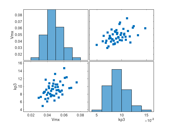
Visualize the sample values.
sTbl2 = generate(sObj);
[s,ax,bigax,h,hax] = plotmatrix([sTbl2.Vmx,sTbl2.kp3]);
ax(1,1).YLabel.String = "Vmx";
ax(2,1).YLabel.String = "kp3";
ax(2,1).XLabel.String = "Vmx";
ax(2,2).XLabel.String = "kp3";
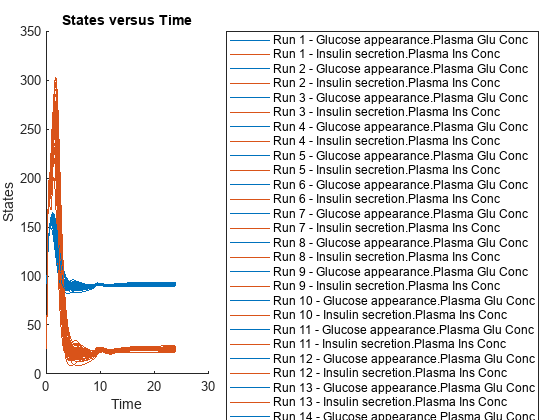
Simulate the scenarios.
sd3 = f(sObj,24);
sbioplot(sd3);
Restore warning settings.
warning(warnSettings);
Input Arguments
Output Arguments
Version History
Introduced in R2019b