sbiompgsa

Perform multiparametric global sensitivity analysis (requires Statistics and Machine Learning Toolbox)

Syntax

mpgsaResults = sbiompgsa(modelObj,params,classifiers)

mpgsaResults = sbiompgsa(modelObj,samples,classifiers)

mpgsaResults = sbiompgsa(modelObj,scenarios,classifiers)

mpgsaResults = sbiompgsa(simdata,samples,classifiers)

mpgsaResults = sbiompgsa(simdata,scenarios,classifiers)

mpgsaResults = sbiompgsa(___,Name,Value)

Description

mpgsaResults = sbiompgsa(modelObj,params,classifiers) performs a multiparametric global sensitivity analysis (MPGSA) [1] of classifiers with respect to model parameters params on a SimBiology model modelObj. params are model quantities (sensitivity inputs) and classifiers define the expressions of model responses (model outputs).

mpgsaResults = sbiompgsa(modelObj,samples,classifiers) uses parameter samples to perform a multiparametric global sensitivity analysis of classifiers.

mpgsaResults = sbiompgsa(modelObj,scenarios,classifiers) draws samples from scanarios, a SimBiology.Scenarios object, to perform the analysis.

mpgsaResults = sbiompgsa(simdata,samples,classifiers) uses model simulation data simdata to perform a multiparametric global sensitivity analysis of classifiers.

mpgsaResults = sbiompgsa(simdata,scenarios,classifiers) uses samples specified in scenarios, a SimBiology.Scenarios object.

mpgsaResults = sbiompgsa(___,Name,Value) uses additional options specified by one or more name-value pair arguments. Available name-value arguments differ depending on which syntax you are using.

Examples

Perform Multiparametric Global Sensitivity Analysis (MPGSA)

Load the target-mediated drug disposition (TMDD) model.

sbioloadproject tmdd_with_TO.sbproj

Get the active configset and set the target occupancy (TO) as the response.

cs = getconfigset(m1);
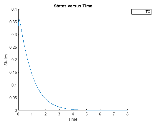
cs.RuntimeOptions.StatesToLog = 'TO';

Simulate the model and plot the TO profile.

sbioplot(sbiosimulate(m1,cs));

Define an exposure (area under the curve of the TO profile) threshold for the target occupancy.

classifier = 'trapz(time,TO) <= 0.1';

Perform MPGSA to find sensitive parameters with respect to the TO. Vary the parameter values between predefined bounds to generate 10,000 parameter samples.

% Suppress an information warning that is issued during simulation.
warnSettings = warning('off', 'SimBiology:sbservices:SB_DIMANALYSISNOTDONE_MATLABFCN_UCON');
rng(0,'twister'); % For reproducibility
params = {'kel','ksyn','kdeg','km'};
bounds = [0.1, 1; 
          0.1, 1;
          0.1, 1;
          0.1, 1];
mpgsaResults = sbiompgsa(m1,params,classifier,Bounds=bounds,NumberSamples=10000)

mpgsaResults = 
  MPGSA with properties:

                    Classifiers: {'trapz(time,TO) <= 0.1'}
    KolmogorovSmirnovStatistics: [4×1 table]
                       ECDFData: {4×4 cell}
              SignificanceLevel: 0.0500
                        PValues: [4×1 table]
              SupportHypothesis: [10000×1 table]
               ParameterSamples: [10000×4 table]
                    Observables: {'TO'}
                 SimulationInfo: [1×1 struct]

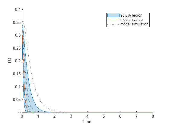
Plot the quantiles of the simulated model response.

plotData(mpgsaResults,ShowMedian=true,ShowMean=false);

Plot the empirical cumulative distribution functions (eCDFs) of the accepted and rejected samples. Except for km, none of the parameters shows a significant difference in the eCDFs for the accepted and rejected samples. The km plot shows a large Kolmogorov-Smirnov (K-S) distance between the eCDFs of the accepted and rejected samples. The K-S distance is the maximum absolute distance between two eCDFs curves.

h = plot(mpgsaResults);
% Resize the figure.
pos = h.Position(:);
h.Position(:) = [pos(1) pos(2) pos(3)*2 pos(4)*2];

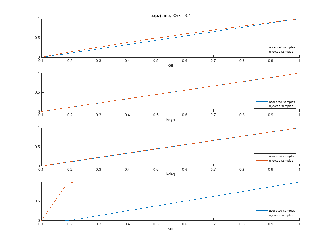
To compute the K-S distance between the two eCDFs, SimBiology uses a two-sided test based on the null hypothesis that the two distributions of accepted and rejected samples are equal. See kstest2 (Statistics and Machine Learning Toolbox) for details. If the K-S distance is large, then the two distributions are different, meaning that the classification of the samples is sensitive to variations in the input parameter. On the other hand, if the K-S distance is small, then variations in the input parameter do not affect the classification of samples. The results suggest that the classification is insensitive to the input parameter. To assess the significance of the K-S statistic rejecting the null-hypothesis, you can examine the p-values.

bar(mpgsaResults)

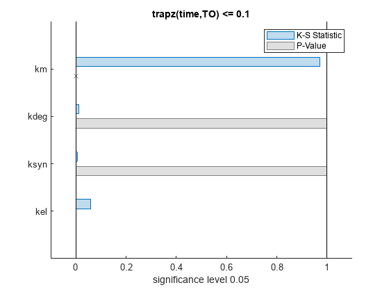
The bar plot shows two bars for each parameter: one for the K-S distance (K-S statistic) and another for the corresponding p-value. You reject the null hypothesis if the p-value is less than the significance level. A cross (x) is shown for any p-value that is almost 0. You can see the exact p-value corresponding to each parameter.

[mpgsaResults.ParameterSamples.Properties.VariableNames',mpgsaResults.PValues]

ans=4×2 table
      Var1      trapz(time,TO) <= 0.1
    ________    _____________________

    {'kel' }          0.0021877      
    {'ksyn'}                  1      
    {'kdeg'}            0.99983      
    {'km'  }                  0      

The p-values of km and kel are less than the significance level (0.05), supporting the alternative hypothesis that the accepted and rejected samples come from different distributions. In other words, the classification of the samples is sensitive to km and kel but not to other parameters (kdeg and ksyn).

You can also plot the histograms of accepted and rejected samples. The historgrams let you see trends in the accepted and rejected samples. In this example, the histogram of km shows that there are more accepted samples for larger km values, while the kel histogram shows that there are fewer rejected samples as kel increases.

h2 = histogram(mpgsaResults);
% Resize the figure.
pos = h2.Position(:);
h2.Position(:) = [pos(1) pos(2) pos(3)*2 pos(4)*2];

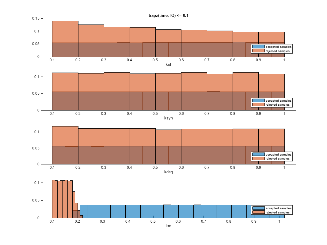
Restore the warning settings.

warning(warnSettings);

Input Arguments

modelObj — SimBiology model

SimBiology model object

SimBiology model, specified as a SimBiology model object.

params — Names of model parameters, species, or compartments

character vector | string | string vector | cell array of character vectors

Names of model parameters, species, or compartments, specified as a character vector, string, string vector, or cell array of character vectors.

Example: ["k1","k2"]

Data Types: char | string | cell

simdata — Model simulation data

vector of SimData objects

Model simulation data, specified as a vector of SimData objects.

scenarios — Source for drawing samples

SimBiology.Scenarios object

Source for drawing samples, specified as a SimBiology.Scenarios object.

Note

The object must not contain doses or variants as its entries.

classifiers — Expressions of model responses

character vector | string | string vector | cell array of character vectors

Expressions of model responses, specified as a character vector, string, string vector, or cell array of character vectors. Specify expressions referencing simulated model quantities, observables, time, or MATLAB functions that are on the path.

Each classifier must evaluate to a logical vector of the same length as the number of parameter samples. Entities, such as model quantities or observables, referenced in a classifier expression are evaluated as a matrix with columns containing time courses of the simulated quantity values. Each column represents one sample. Each row represents one output time. For details, see Multiparametric Global Sensitivity Analysis (MPGSA).

If you specify a SimData object as the first input, each quantity or observable referenced by the classifier must resolve to a logged component in the SimData object.

You can formulate a classifier as a modeling question such as whether a model parameter have an effect on the model response exceeding or falling below a target threshold. For example, the following classifier defines an exposure (area under the curve) threshold for the target occupancy TO: trapz(time,TO) <= 0.1. Another classifier, used by the authors in [1], measures the deviation of the averaged model response from the mean model response over the parameter domain: mean(TO,1) < mean(TO,'all'). Here mean(TO,1) computes the averaged model response across time for each sample of the sensitivity inputs, and mean(TO,'all') computes the mean value of the TO response across all output times and all samples.

Example: "max(Central.Drug(time > 1,:),[],1) <= 7"

Data Types: char | string | cell

samples — Sampled values of model quantities

table

Sampled values of model quantities, specified as a table. The variable names of the table indicate the quantity names.

Data Types: table

Name-Value Arguments

Example: mpgsaResults = sbiompgsa(m1,{'k1','k2'},classifier,'Bounds',[0.5 5;0.1 1]) specifies parameter bounds for k1 and k2.

Specify one or more comma-separated pairs of Name,Value arguments. Name is the argument name and Value is the corresponding value. Name must appear inside quotes. You can specify several name and value pair arguments in any order as Name1,Value1,...,NameN,ValueN.

Note

Depending on which syntax you use, available name-value pairs differ.

For the First Syntax

Bounds — Parameter bounds

numeric matrix

Parameter bounds, specified as a numeric matrix with two columns. The first column contains the lower bounds and the second column contains the upper bounds. The number of rows must be equal to the number of parameters in params.

If a parameter has a nonzero value, the default bounds are ±10% of the value. If the parameter value is zero, the default bounds are [0 1].

Example: [0.5 5]

Data Types: double

NumberSamples — Number of samples drawn to perform multiparametric global sensitivity analysis

1000 (default) | positive integer

Number of samples drawn to perform multiparametric global sensitivity analysis, specified as the comma-separated pair consisting of 'NumberSamples' and a positive integer.

Data Types: double

SamplingMethod — Method to generate parameter samples

'Sobol' (default) | character vector | string

Method to generate parameter samples, specified as a character vector or string. Valid options are:

• 'Sobol' — Use the low-discrepancy Sobol sequence to generate samples.

• 'Halton' — Use the low-discrepancy Halton sequence to generate samples.

• 'lhs' — Use the low-discrepancy Latin hypercube samples.

• 'random' — Use uniformly distributed random samples.

Data Types: char | string

SamplingOptions — Options for sampling method

struct

Options for the sampling method, specified as a scalar struct. The options differ depending on the sampling method: sobol, halton, or lhs.

For sobol and halton, specify each field name and value of the structure according to each name-value argument of the sobolset (Statistics and Machine Learning Toolbox) or haltonset (Statistics and Machine Learning Toolbox) function. SimBiology uses the default value of 1 for the Skip argument for both methods. For all other name-value arguments, the software uses the same default values of sobolset or haltonset. For instance, set up a structure for the Leap and Skip options with nondefault values as follows.

s1.Leap = 50;
s1.Skip = 0;

For lhs, there are three samplers that support different sampling options.

• If you specify a covariance matrix, SimBiology uses lhsnorm (Statistics and Machine Learning Toolbox) for sampling. SamplingOptions argument is not allowed.

• Otherwise, use the field name UseLhsdesign to select a sampler.

  • If the value is true, SimBiology uses lhsdesign (Statistics and Machine Learning Toolbox). You can use the name-value arguments of lhsdesign to specify the field names and values.

  • If the value is false (default), SimBiology uses a nonconfigurable Latin hypercube sampler that is different from lhsdesign. This sampler does not require Statistics and Machine Learning Toolbox™. SamplingOptions cannot contain any other options, except UseLhsdesign.

For instance, set up a structure to use lhsdesign with the Criterion and Iterations options.

s2.UseLhsdesign  = true;
s2.Criterion     = "correlation";
s2.Iterations    = 10;

You cannot specify this argument when a SimBiology.Scenarios object is an input.

sbiompgsa ignores this argument if you are also specifying a table of samples as the second input.

Distributions — Probability distributions

prob.UniformDistribution (default) | prob.ProbabilityDistribution object | vector of prob.ProbabilityDistribution objects

Probability distributions used to draw samples, specified as a prob.ProbabilityDistribution object or vector of these objects. Specify a scalar prob.ProbabilityDistribution or vector of length N, where N is the number of input parameters. You can create distribution objects to sample from various distributions, such as uniform, normal, or lognormal distributions, using makedist (Statistics and Machine Learning Toolbox).

If you specify a scalar prob.ProbabilityDistribution object, and there are multiple input parameters, sbiompgsa uses the same distribution object to draw samples for each parameter.

You cannot specify this argument together with Bounds.

You cannot specify this argument when a SimBiology.Scenarios object is an input.

sbiompgsa ignores this argument when a table of samples is an input.

For the First and Second Syntaxes

Doses — Doses to use during simulations

ScheduleDose object | RepeatDose object | vector of dose objects

Doses to use during model simulations, specified as a ScheduleDose or RepeatDose object or a vector of dose objects.

Variants — Variants to apply before simulations

variant object | vector of variant objects

Variants to apply before model simulations, specified as a variant object or vector of variant objects.

When you specify multiple variants with duplicate specifications for a property's value, the last occurrence for the property value in the array of variants is used during simulation.

StopTime — Simulation stop time

nonnegative scalar

Simulation stop time, specified as a nonnegative scalar. If you specify neither StopTime nor OutputTimes, the function uses the stop time from the active configuration set of the model. You cannot specify both StopTime and OutputTimes.

Data Types: double

UseParallel — Flag to run model simulations in parallel

false (default) | true

Flag to run model simulations in parallel, specified as true or false. When the value is true and Parallel Computing Toolbox™ is available, the function runs simulations in parallel.

Data Types: logical

Accelerate — Flag to turn on model acceleration

true (default) | false

Flag to turn on model acceleration, specified as true or false.

Data Types: logical

For All Syntaxes

OutputTimes — Simulation output times

numeric vector

Simulation output times, specified as the comma-separated pair consisting of 'OutputTimes' and a numeric vector. The function computes model responses at these output time points. You cannot specify both StopTime and OutputTimes. By default, the function uses the output times of the first model simulation.

Example: [0 1 2 3.5 4 5 5.5]

Data Types: double

SignificanceLevel — Significance level for Kolmogorov-Smirnov test

0.05 (default) | numeric scalar between 0 and 1

Significance level for Kolmogorov-Smirnov test, specified as the comma-separated pair consisting of 'SignificanceLevel' and a numeric scalar between 0 and 1. For details, see Two-Sample Kolmogorov-Smirnov Test (Statistics and Machine Learning Toolbox).

Example: 0.1

Data Types: double

InterpolationMethod — Method for interpolation of model simulations

"interp1q" (default) | character vector | string

Method for interpolation of model responses to a common set of output times, specified as a character vector or string. The valid options follow.

• "interp1q" — Use the interp1q function.

• Use the interp1 function by specifying one of the following methods:

  • "nearest"

  • "linear"

  • "spline"

  • "pchip"

  • "v5cubic"

• "zoh" — Specify zero-order hold.

Data Types: char | string

Output Arguments

mpgsaResults — Multiparametric global sensitivity analysis results

SimBiology.gsa.MPGSA object

Multiparametric global sensitivity analysis results, returned as a SimBiology.gsa.MPGSA object. The object also contains model simulation data used to perform MPGSA.

More About

Multiparametric Global Sensitivity Analysis (MPGSA)

Multiparametric global sensitivity analysis lets you study the relative importance of parameters with respect to a classifier defined by model responses. A classifier is an expression of model responses that evaluates to a logical vector. sbiompgsa implements the MPSA method described by Tiemann et. al. (see supporting information text S2) [1].

sbiompgsa performs the following steps.

1. Generate N parameter samples using a sampling method. sbiompgsa stores these samples as a table in a property, mpgsaResults.ParameterSamples, of the returned object. The number of rows is equal to the number of samples and the number of columns is equal to the number of input parameters.

   Tip

   You can specify N and the sampling method using the 'NumberSamples' and 'SamplingMethod' name-value pair arguments, respectively, when you call sbiompgsa.

2. Calculate the model response by simulating the model for each parameter set, which is a single realization of the model parameter values. In this case, a parameter set is equal to a row in the ParameterSamples table.

3. Evaluate the classifier. A classifier is an expression that evaluates to a logical vector. For instance, if your model response is the AUC of plasma drug concentration, you can define a classifier with a toxicity threshold of 0.8 where the AUC of the drug concentration above that threshold is considered toxic.

4. Parameter sets are then separated into two different groups, such as accepted (nontoxic) and rejected (toxic) groups.

5. For each input parameter, compute the empirical cumulative distribution functions (ecdf (Statistics and Machine Learning Toolbox)) of accepted and rejected sample values.

6. Compare the two eCDFs of accepted and rejected groups using the Two-Sample Kolmogorov-Smirnov Test (Statistics and Machine Learning Toolbox) to compute the Kolmogorov-Smirnov distance. The default significance level of the Kolmogorov-Smirnov test is 0.05. If two eCDFs are similar, the distance is small, meaning the model response is not sensitive with respect to the input parameter. If two eCDFs are different, the distance is large, meaning the model response is sensitive to the parameter.

   Note

   The Kolmogorov-Smirnov test assumes that the samples follow a continuous distribution. Make sure that the eCDF plots are continuous as you increase the number of samples. If eCDFs are not continuous but step-like in the limit of infinite samples, then the results might not reflect the true sensitivities.

References

[1] Tiemann, Christian A., Joep Vanlier, Maaike H. Oosterveer, Albert K. Groen, Peter A. J. Hilbers, and Natal A. W. van Riel. “Parameter Trajectory Analysis to Identify Treatment Effects of Pharmacological Interventions.” Edited by Scott Markel. PLoS Computational Biology 9, no. 8 (August 1, 2013): e1003166. https://doi.org/10.1371/journal.pcbi.1003166.

Version History

Introduced in R2020a