rpmtrack
Track and extract RPM profile from vibration signal
Syntax
Description
rpm = rpmtrack(x,fs,order,p)rpm from a vibration signal x
sampled at a rate fs.
The two-column matrix p contains a set of points that lie
on a time-frequency ridge corresponding to a given order.
Each row of p specifies one coordinate pair. If you call
rpmtrack without specifying both
order and p, the function opens an
interactive plot that displays the time-frequency map and enables you to select
the points.
If you have a tachometer pulse signal, use tachorpm to extract
rpm directly.
rpm = rpmtrack(___,Name=Value)
rpmtrack(___) with no output arguments plots
the power time-frequency map and the estimated RPM profile on an interactive
figure.
Examples
Generate a vibration signal with three harmonic components. The signal is sampled at 1 kHz for 16 seconds. The signal's instantaneous frequency resembles the runup and coastdown of an engine. Compute the instantaneous phase by integrating the frequency using the trapezoidal rule.
fs = 1000;
t = 0:1/fs:16;

ifq = 20 + t.^6.*exp(-t);
phi = 2*pi*cumtrapz(t,ifq);
The harmonic components of the signal correspond to orders 1, 2, and 3. The order-2 sinusoid has twice the amplitude of the others.
ol = [1 2 3];
amp = [5 10 5];

vib = amp*cos(ol'.*phi);
Extract and visualize the RPM profile of the signal using a point on the order-2 ridge.
time = 3;
order = 2;
p = [time order*ifq(t==time)];

rpmtrack(vib,fs,order,p)
Generate a signal that resembles the vibrations caused by revving a car engine. The signal is sampled at 1 kHz for 30 seconds and contains three harmonic components of orders 1, 2.4, and 3, with amplitudes 5, 4, and 0.5, respectively. Embed the signal in unit-variance white Gaussian noise and store it in a MATLAB® timetable. Multiply the instantaneous frequency by 60 to obtain an RPM profile. Plot the RPM profile.
fs = 1000;
t = (0:1/fs:30)';

fit = @(a,x) (t-x).^6.*exp(-(t-x)).*((t-x)>=0)*a';

fis = fit([0.4 1 0.6 1],[0 6 13 17]);
phi = 2*pi*cumtrapz(t,fis);

ol = [1 2.4 3];
amp = [5 4 0.5]';
vib = cos(phi.*ol)*amp + randn(size(t));

xt = timetable(seconds(t),vib);

plot(t,fis*60)

Derive the RPM profile from the vibration signal. Use four points at 5 second intervals to specify the ridge corresponding to order 2.4. Display a summary of the output timetable.
ndx = (5:5:20)*fs;
order = ol(2);

p = [t(ndx) order*fis(ndx)];

rpmest = rpmtrack(xt,order,p);

summary(rpmest)
rpmest: 30001×1 timetable

Row Times:

    tout: duration

Variables:

    rpm: double

Statistics for applicable variables and row times:

            NumMissing         Min              Median             Max               Mean              Std

    tout        0           0 sec             15 sec            30 sec            15 sec            8.6607 sec
    rpm         0           2.2204e-16        4.3272e+03        8.8798e+03        4.2732e+03        2.5558e+03
Plot the reconstructed RPM profile and the points used in the reconstruction.
hold on
plot(seconds(rpmest.tout),rpmest.rpm,'.-')
plot(t(ndx),fis(ndx)*60,'ok')
hold off
legend('Original','Reconstructed','Ridge points','Location','northwest')

Use the extracted RPM profile to generate the order-RPM map of the signal.
rpmordermap(vib,fs,rpmest.rpm)

Reconstruct and plot the time-domain waveforms that compose the signal. Zoom in on a time interval occurring after the transients have decayed.
xrc = orderwaveform(vib,fs,rpmest.rpm,ol);

figure
plot(t,xrc)
legend([repmat('Order = ',[3 1]) num2str(ol')])
xlim([5 20])
Estimate the RPM profile of a fan blade as it slows down after switchoff.
An industrial roof fan spinning at 20,000 rpm is turned off. Air resistance (with a negligible contribution from bearing friction) causes the fan rotor to stop in approximately 6 seconds. A high-speed camera measures the x-coordinate of one of the fan blades at a rate of 1 kHz.
fs = 1000;
t = 0:1/fs:6-1/fs;

rpm0 = 20000;
Idealize the fan blade as a point mass circling the rotor center at a radius of 50 cm. The blade experiences a drag force proportional to speed, resulting in the following expression for the phase angle
where is the initial frequency and second is the decay time.
a = 0.5;
f0 = rpm0/60;
T = 0.75;

phi = 2*pi*f0*T*(1-exp(-t/T));
Compute and plot the x- and y-coordinates of the blade. Add white Gaussian noise of variance .
x = a*cos(phi) + randn(size(phi))/10;
y = a*sin(phi) + randn(size(phi))/10;

plot(t,x,t,y)
xlabel("Time (s)")
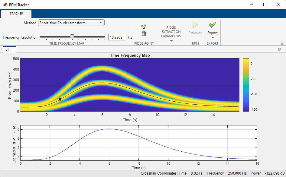
Use the rpmtrack function to determine the RPM profile. Type this command to open the interactive figure.
rpmtrack(x,fs)

Use the slider to adjust the frequency resolution of the time-frequency map to about 11 Hz. Assume that the signal component corresponds to order 1 and set the end time for ridge extraction to 3.0 seconds. Use the crosshair cursor in the time-frequency map and the Add button to add three points lying on the ridge. Alternatively, double-click the cursor to add the points at the locations you choose. Click Estimate to track and extract the RPM profile.

Verify that the RPM profile decays exponentially. On the Export tab, click Export and select Generate MATLAB Script. The script appears in the Editor.
% MATLAB Code from rpmtrack GUI

% Generated by MATLAB 9.12 and Signal Processing Toolbox 8.7

% Generated on 12-Oct-2021 09:36:49

% Set sample rate
fs = 1000.0000;
% Set order of ridge of interest
order = 1.0000;
% Set ridge points on ridge of interest
ridgePoints = [...
    0.4077 194.6023;...
    0.9781 89.4886;...
    2.3678 15.6250];
% Estimate RPM
[rpmOut,tOut] = rpmtrack(x,fs,order,ridgePoints,...
    'Method','stft',...
    'FrequencyResolution',11.1612,...
    'PowerPenalty',Inf,...
    'FrequencyPenalty',0.0000,...
    'StartTime',0.0000,...
    'EndTime',3.0000);
Run the script. Display the RPM profile in a semilogarithmic plot.
semilogy(tOut,rpmOut)
ylim([500 20000])
xlabel("Time (s)")
Input Arguments
Name-Value Arguments
Output Arguments
Algorithms
rpmtrack uses a two-step (coarse-fine) estimation method:
Compute a time-frequency map of
xand extract a time-frequency ridge based on a specified set of points on the ridge,p, theordercorresponding to that ridge, and the optional penalty parametersPowerPenaltyandFrequencyPenalty. The extracted ridge provides a coarse estimate of the RPM profile.Compute the order waveform corresponding to the extracted ridge using a Vold-Kalman filter and calculate a new time-frequency map from this waveform. The isolated order ridge from the new time-frequency map provides a fine estimate of the RPM profile.
References
[1] Urbanek, Jacek, Tomasz Barszcz, and Jerome Antoni. "A Two-Step Procedure for Estimation of Instantaneous Rotational Speed with Large Fluctuations." Mechanical Systems and Signal Processing. Vol. 38, 2013, pp. 96–102.
Extended Capabilities
Version History
Introduced in R2018a