Plan Collision-Free Path for Excavator Arm in MATLAB With Lidar Data
This example shows how to plan a collision-free path for an excavator arm in an environment that may contain obstacles.
For this example, use Lidar data to represent the environment and to create an occupancy map. The occupancy map helps the planner in creating a collision-free path between a start and goal pose of the excavator arm.
See the Simulate Earth Moving with Autonomous Excavator in Construction Site example to use this collision-free path to simulate an excavator model in Unreal.
This example uses the following toolboxes:
Robotics System Toolbox™ — Model an excavator using
rigidBodyTreemanipulatorRRT.Navigation Toolbox™ — Represent the environment as an occupancy map with the
occupancyMap3D(Navigation Toolbox)Optimization Toolbox™ — Generate the trajectory using the
contopptraj
Initial Setup
Load the Excavator Model
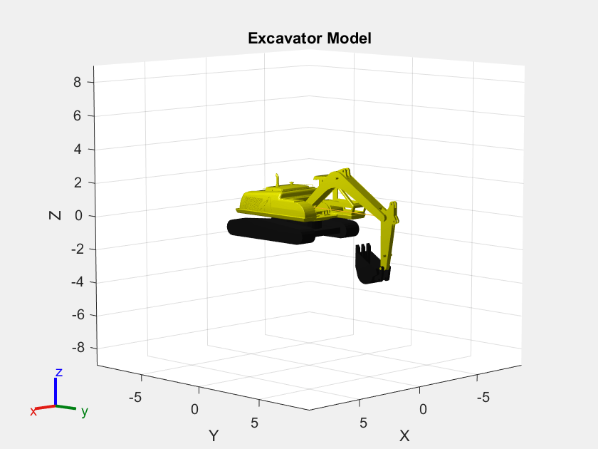
Load the rigidBodyTree model of the excavator from the provided MAT file MathScavator9000.mat. This model of the excavator was created using a CAD software and then exported to the URDF format. The URDF and the associated meshes were then imported to MATLAB using the importrobot function to create the rigidBodyTree model.
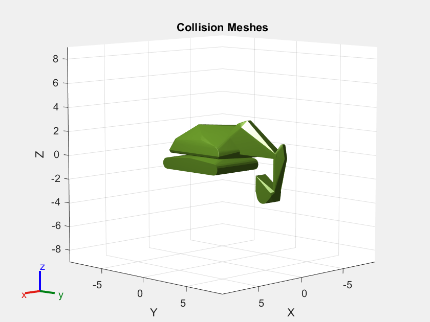
The model contains visual and collision meshes of the excavator model. The motion planner uses the collision meshes to ensure a collision-free path.
load MathScavator9000.mat
show(excavatorRBT);
title("Excavator Model")
show(excavatorRBT, Collisions="on", Visuals="off");
title("Collision Meshes")
In the Lidar data set, positive x-axis points in the forward direction of the excavator. In the rigidBodyTree model, the positive y-axis points in the forward direction of the excavator. Rotate the rigidBodyTree model by -90 degrees around the z-axis so that the orientation of the rigidBodyTree model matches the orientation specified in the Lidar data set. The helper function exampleHelperSetRigidBodyTreeRotation adds a rotating body with a fixed joint that offsets the base of the excavator from the world frame by -90 degrees along the z-axis.
tform = eul2tform([-pi/2,0,0]);
excavatorRBT = exampleHelperSetRigidBodyTreeRotation(excavatorRBT, tform);
excavatorRBT.DataFormat = 'row';
show(excavatorRBT);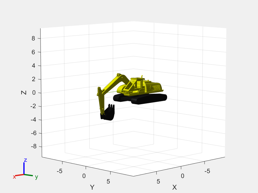
To ensure that the excavator bucket doesn't open up to drop the payload during the planned motion, we adjust the stick to bucket joint limits for this motion planning problem. Adjust the boom to stick and chassis to stick joint limits to get a more desirable path for the excavator arm.
excavatorRBT.getBody("stick_bucket_link").Joint.PositionLimits = [0 0.2];
excavatorRBT.getBody("boom_stick_link").Joint.PositionLimits(2) = 0.5;
excavatorRBT.getBody("chassis_boom_link").Joint.PositionLimits(2) = 0.9;
Modify Collision Mesh
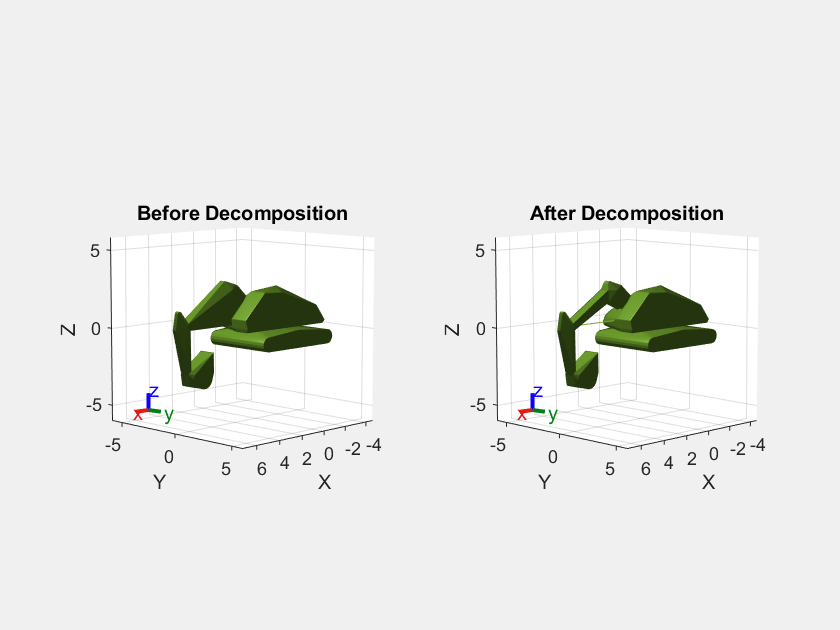
The goal of this example is to modify the collision meshes to get a collision model that is adequate for motion planning while keeping the number of meshes to a minimum. The model includes collision meshes that are convex hulls of the visual meshes, which are not optimal for collision checking as they tend to be bulky.
Remove the collision mesh from the base because the excavator in this example is stationary. This mesh collides with the map and removing it does not affect the motion planning of the arm.
clearCollision(excavatorRBT.Base);
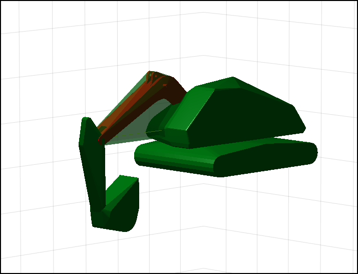
The collision mesh for the boom is too conservative as it fits a convex hull around the concave visual mesh. This mesh may restrict the motion planner from traversing valid solutions. This image details the issue.
Decompose Visual Mesh
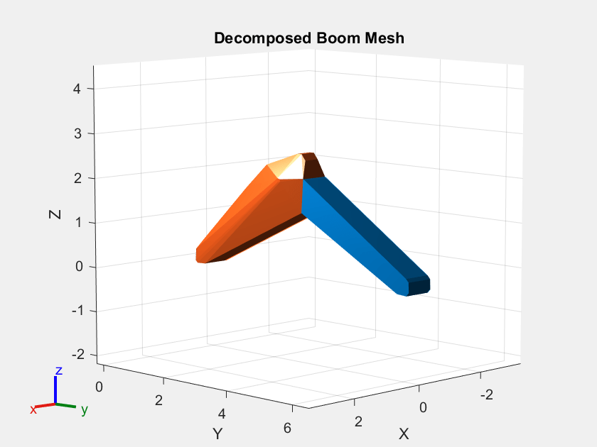
Decompose the boom mesh to get several smaller convex meshes that offer a more accurate representation.
Get the boom body and its visual mesh.
boomBody = getBody(excavatorRBT, 'chassis_boom_link');
visData = getVisual(boomBody);
Decompose the visual mesh using collisionVHACD. Define the vhacdOptions to create a maximum of two convex hulls of the boom mesh.
opts = vhacdOptions("IndividualMesh", "MaxNumConvexHulls",2);
collisionArray = collisionVHACD(visData(1).Triangulation,opts);
Visualize the decomposed meshes to verify that they are an improvement over the previous mesh.
showCollisionArray(collisionArray)
ans =
  Axes with properties:

             XLim: [-3.3468 3.3547]
             YLim: [-0.2218 6.4797]
           XScale: 'linear'
           YScale: 'linear'
    GridLineStyle: '-'
         Position: [0.1300 0.1100 0.7750 0.8150]
            Units: 'normalized'

  Show all properties
title("Decomposed Boom Mesh")
drawnow
Clear the existing collision mesh from the boom body and add the convex meshes obtained from the decomposition.
excavatorOriginal = copy(excavatorRBT);
clearCollision(boomBody);

cellfun(@(x)boomBody.addCollision(x), collisionArray);

tiledlayout(1,2);
nexttile(1)
show(excavatorOriginal, Visuals="off", Collisions="on");
title("Before Decomposition")
axis auto
nexttile(2)
show(excavatorRBT, Visuals="off", Collisions="on");
title("After Decomposition")
axis auto
You can decompose the convex mesh when you import the model by using the CollisionDecomposition name-value argument. For more information, see the "Decompose Collision Meshes of Imported Robot" example in the importrobot documentation.
Create Environment Occupancy Map
The game engine provides the Lidar data of the environment. However, this Lidar data contains points that belong to the excavator on which the Lidar sensors are placed. Clean this data so that it contains only the points belonging to the environment.
For more information on how to clean the data set, see the Extract Scene From Lidar Data example.
For this example, we use the cleaned up data stored in a MAT file. Load the MAT file containng the environment data.
load environmentPoints.matRepresent the environment using an occupancyMap3D object and specify that object as an input to the planner.
omap3D = occupancyMap3D(10);
pose = [0 0 0 1 0 0 0];

maxRange = double( max(envPoints, [], 'all') );
insertPointCloud(omap3D, pose, envPoints, maxRange)
figure;
show(omap3D)
axis equal
![Figure contains an axes object. The axes object with title Occupancy Map, xlabel X [meters], ylabel Y [meters] contains an object of type patch.](../../examples/offroad_autonomy/win64/PlanExcavatorArmMotionInMATLABWithLidarDataExample_07.png)
Path Planning
Create Motion Planner
Create a motion planner using one of the planners for rigidBodyTree objects. This example leverages the manipulatorRRT planner, which is a sampling-based planner for rigidBodyTree objects. You can find other planners in Manipulator Planning.
Tune the MaxConnectionDistance and ValidationDistance to the task. For more details on how various parameters affect the planner see the documentation on manipulatorRRT or this Pick-and-Place Workflow Using RRT for Manipulators.
The valid motion range of the arm is already constrained by the joint limits. Set the planner to skip self collision between bodies that have a parent relation by setting SkippedSelfCollisions to "parent".
Create the planner object with the above options.
planner = manipulatorRRT(excavatorRBT, {}, Map=omap3D, MaxConnectionDistance=1, ValidationDistance=0.03, SkippedSelfCollisions="parent");Set Up Planning Problem
Define the start and goal poses of the excavator arm. In this example, the initial state places the excavator arm after it grabs a bucket of soil, and the target state places the excavator arm where it drops the soil into a container.
initialState = deg2rad([0 -8 50 0]);
targetState = deg2rad([120 45 20 0]);
Visualize the environment and the start and the goal poses of the excavator arm.
show(excavatorRBT,initialState);
hold on
show(omap3D)
view(45, 30)
axis equal
hold off
title("Initial State")
![Figure contains an axes object. The axes object with title Initial State, xlabel X [meters], ylabel Y [meters] contains 19 objects of type patch, line. These objects represent base, baseRotator, base_link, base_chassis_link, chassis_boom_link, boom_stick_link, stick_bucket_link, base_link_mesh, base_chassis_link_mesh, chassis_boom_link_mesh, boom_stick_link_mesh, stick_bucket_link_mesh.](../../examples/offroad_autonomy/win64/PlanExcavatorArmMotionInMATLABWithLidarDataExample_08.png)
show(excavatorRBT,targetState);
hold on
show(omap3D)
view(45, 30)
axis equal
hold off
title("Target State")
![Figure contains an axes object. The axes object with title Target State, xlabel X [meters], ylabel Y [meters] contains 19 objects of type patch, line. These objects represent base, baseRotator, base_link, base_chassis_link, chassis_boom_link, boom_stick_link, stick_bucket_link, base_link_mesh, base_chassis_link_mesh, chassis_boom_link_mesh, boom_stick_link_mesh, stick_bucket_link_mesh.](../../examples/offroad_autonomy/win64/PlanExcavatorArmMotionInMATLABWithLidarDataExample_09.png)
Plan Collision-Free Path
To obtain a collision-free path, run the planner with the initial and target states as inputs.
rng(20); % For repeatability (optional)
path = plan(planner,initialState,targetState);
Given the planner design, the initial path returned by it may be inefficient and can appear somewhat random. Smooth the results by interpolating between the planned poses.
smoothPath = interpolate(planner, path, 5);
Animate the planned path in MATLAB. This output shows the outcome of the planner using the simplified model and environment.
ax = show(excavatorRBT,initialState,Collisions="off");
zlim([-4 10])

hold on
show(omap3D,Parent=ax);
view(70, 30)

% Animate the planned path
rc = rateControl(10);
for ii = 1:size(smoothPath,1)
    show(excavatorRBT,smoothPath(ii,:),Parent=ax,Collisions="off",FastUpdate=true,PreservePlot=false);
    waitfor(rc);
end
hold off

Path to Trajectory Conversion
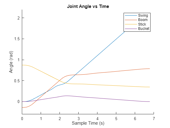
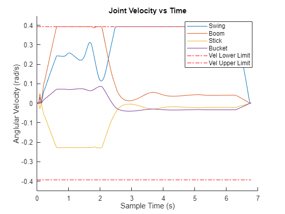
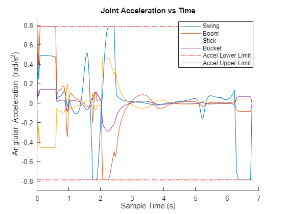
The path that the planner generates is time independent. To easily control the motion, you must associate the simulation time with the path such that you can provide a reference trajectory to the position-controlled excavator. While there are several polynomial trajectory blocks that you can use, the contopptraj function enables you to generate a trajectory by specifying velocity and acceleration limits for the excavator joints in addition to the waypoints.
velocityLimits = repmat([-pi/8, pi/8], 4, 1);
accelerationLimits = repmat([-pi/4, pi/4], 4, 1);
[q, qd, qdd, t] = contopptraj(smoothPath', velocityLimits, accelerationLimits, "NumSamples", 200);
Plot the position, velocity, and acceleration of each joint of the excavator arm against time. Draw the upper and lower velocity and acceleration limits to verify that they are not violated. The provided helper exampleHelperPlotData creates these plots.
exampleHelperPlotData(t, q, qd, qdd, velocityLimits, accelerationLimits);
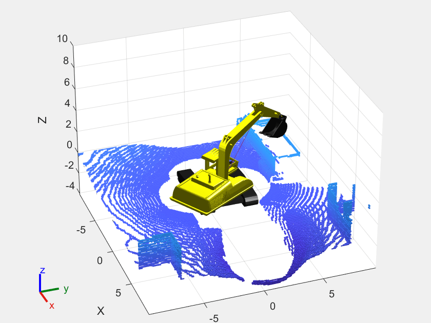
Animate the motion of the excavator arm along the trajectory.
ax = show(excavatorRBT,initialState,Collisions="off");
zlim([-4 10])
hold on
show(omap3D,Parent=ax);
view(70, 30)

% Animate the excavator along the trajectory
rc = rateControl(10);
for ii = 1:4:size(q',1)
    show(excavatorRBT,q(:,ii)',Parent=ax,Collisions="off",FastUpdate=true,PreservePlot=false);
    waitfor(rc);
end
hold off

Conclusion
This example demonstrated motion planning of an excavator arm rigidBodytree in a collision environment where the environment was modelled using Lidar data. A trajectory was generated from the collision-free path using contopptraj that kept the joint velocity and acceleration within a specified limit.