Design and Simulate an FMCW Long-Range Radar (LRR)
This example shows how to generate measurement-level radar detections using a radarDataGenerator created from a radar design exported from the Radar Designer app. The radar will be able to detect vehicles at ranges greater than 300 meters with sufficient resolution to resolve targets in adjacent lanes at this range. You will also learn how to generate signal-level radar detections using an equivalent radarTransceiver created from the radarDataGenerator. The measurement- and signal-level detections are compared to the system-level design analysis provided by the Radar Designer app.
Design System Parameters and Predict Performance Metrics
Design a long-range automotive radar based on the transmit beamforming (TXBF) design in [1] using the Radar Designer app. To open this design in the app, run the command:
radarDesigner('LRR_RadarDesignerSession.mat')
The system parameters under the Main section in the left-hand panel of the radar designer app come from Table 3 in [1] and Section 8.7 in [2]. In particular, the 26 us sweep repetition interval (or PRI in the app) is calculated as the sum of the FMCW waveform sweep time (17 us), the FMCW transceiver's idle time (4 us) and ADC start time (5 us). The 0.65 duty cycle is the ratio of sweep time over the sweep repetition interval.
The Antenna and scanning parameters are found in Table 1 in [3]. Since arrays are used on both transmit (Tx) and receive (Rx), total transmit and receive gains are calculated as the sum of the antenna element directivity (12 dBi) and the array factor (11 dB for the 12 element Tx array, 12 dB for the 16 element Rx array).
The Detection and Tracking parameters are found in Table 3 in [1] and a typical false alarm rate of 1e-6 is assumed.
A 10 dBsm, non-fluctuating radar cross-section (RCS) target positioned 20 cm above the ground is used for Radar Designer app system-level performance analysis and metrics. This target is representative of a mid-sized sedan for an automotive radar. The target must be detected with a probability of 0.9. The environment losses considered are limited to free space propagation loss.
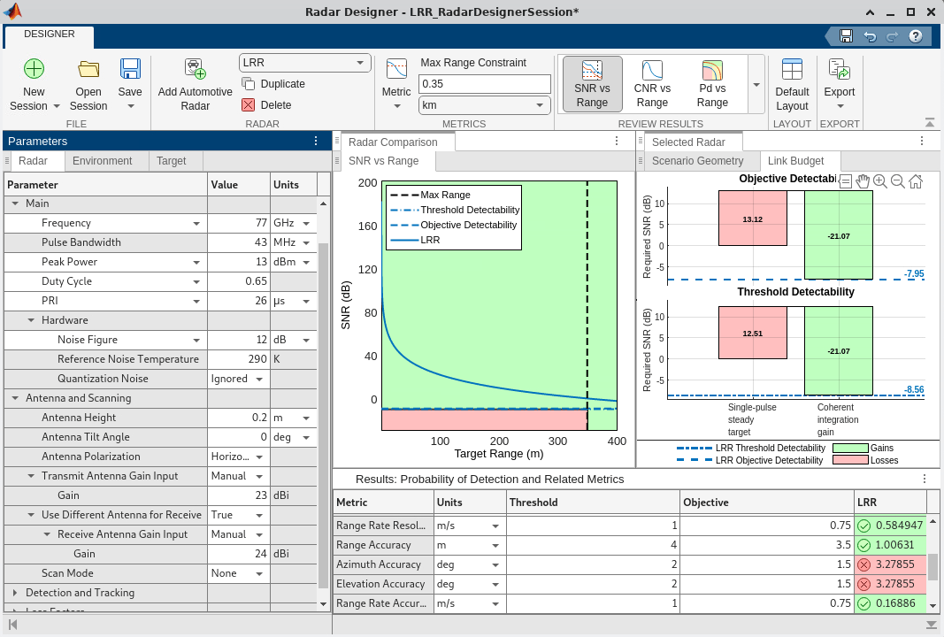
The SNR vs. range plot shows the SNR of a single sweep that's available before any signal processing in the receiver. For a target at approximately 25.4 meters, the single sweep SNR is predicted to be around 47 dB. In addition, the detectability factor charts indicate that the 128 sweeps (or "pulses" on the app) yield a coherent integration gain of 21 dB. Run the range analysis script exported from the app (the plots have been commented out). The script provides an API for the system parameters.
Model the FMCW waveform transceiver's idle and ADC start time using a sweep repetition interval and duty cycle.
LRRRangeAnalysis;
lrrSysParam = radar
lrrSysParam = struct with fields:
                    Name: 'LRR'
        AzimuthBeamwidth: [2×1 double]
      ElevationBeamwidth: [2×1 double]
               Frequency: 7.7000e+10
                    Gain: [23 24]
                  Height: 0.2000
        NoiseTemperature: 4.5962e+03
                 NumCPIs: 1
       NumCoherentPulses: 128
    NumNonCoherentPulses: 1
                     PRF: 38462
               PeakPower: 0.0200
                     Pfa: 1.0000e-06
            Polarization: 'H'
              Pulsewidth: 1.6900e-05
               TiltAngle: 0
              Wavelength: 0.0039
       SystemTemperature: 4.5962e+03
tgtRg = 26; % Target range (m)
singleSweepSNR = interp1(target.ranges,availableSNR,tgtRg)
singleSweepSNR = 46.4857
coherentIntGain = pow2db(lrrSysParam.NumCoherentPulses)
coherentIntGain =
21.0721
predictedSNR = singleSweepSNR + coherentIntGain
predictedSNR =
67.5578
The table at the bottom of the Radar Designer app shows that the predicted performance metrics of the design (right column) meet all threshold requirements (left column) and all objective requirements (middle column) except for the azimuth and elevation accuracy. Run the metrics report script that was also exported from the app to enable comparisons in the following sections. Remove less relevant metrics.
LRRExportedMetricsReport;
predictedLRRMetrics = metricsTable;
predictedLRRMetrics([2:3 12:15],:) = []; % Remove less relevant metrics
Configure a Measurement-Level Model of the Radar
Use the design parameters and metrics exported from the Radar Designer app to configure a radarDataGenerator, which is a measurement-level model that you can use to simulate detections in different scenarios. The model abstracts the detailed signal processing chain and produces detections whose statistics are governed by the desired probabilities of detection and false alarm evaluated for a reference RCS at a reference range corresponding to the detectability threshold.
Fc = lrrSysParam.Frequency;
detThreshold = Dx(2); % Dx is a variable created by the LRRRangeAnalysis script
maxSpd = predictedLRRMetrics{'First Blind Speed',end}/2; % The range-rate limits are [-vb/2, +vb/2), where vb is the blind speed
measLvlLRR = radarDataGenerator(1, 'No scanning', ...
    'DetectionProbability', predictedLRRMetrics{'Probability of Detection',3}, ... % Objective Pd
    'FalseAlarmRate', lrrSysParam.Pfa, ...
    'ReferenceRCS', target.RCS, ...
    'ReferenceRange', interp1(availableSNR,target.ranges,detThreshold,'spline','extrap'), ... % Range at which the SNR crossed the objective detectability threshold
    'MountingLocation', [3.7 0 lrrSysParam.Height], ...
    'CenterFrequency', Fc, ...
    'Bandwidth', rangeres2bw(predictedLRRMetrics{'Range Resolution',end}), ...
    'RangeResolution', predictedLRRMetrics{'Range Resolution',end}, ...
    'HasRangeRate', true, ...
    'RangeRateResolution', predictedLRRMetrics{'Range Rate Resolution',end}, ...
    'RangeLimits', [0 predictedLRRMetrics{'Unambiguous Range',end}], ...
    'RangeRateLimits', [-1 1]*maxSpd, ...
    'HasRangeAmbiguities', true, ...
    'MaxUnambiguousRange', predictedLRRMetrics{'Unambiguous Range',end}, ...
    'HasRangeRateAmbiguities', true, ...
    'MaxUnambiguousRadialSpeed', maxSpd, ...
    'TargetReportFormat', 'Detections', ...
    'DetectionCoordinates', 'Sensor spherical');

rng default % Set random seed for reproducible results
A few parameters required by the radarDataGenerator are not exported by the app. These values are taken from Table 1 and Table 3 in [1] and Table 1 in [3].
4-element series-fed patch azimuth field of view: 120 deg
4-element series-fed patch elevation field of view: 60 deg
Required azimuth resolution: 1.4 deg
Bandwidth: 43 MHz
measLvlLRR.FieldOfView = [120 60];
measLvlLRR.AzimuthResolution = 1.4;
The measurement-level radar is now configured to match the design parameters analyzed in the Radar Designer app.
disp(measLvlLRR)
  radarDataGenerator with properties:

                  SensorIndex: 1
                   UpdateRate: 1
                DetectionMode: 'Monostatic'
                     ScanMode: 'No scanning'
        InterferenceInputPort: 0
           EmissionsInputPort: 0

             MountingLocation: [3.7000 0 0.2000]
               MountingAngles: [0 0 0]

                  FieldOfView: [120 60]
                  RangeLimits: [0 3.8973e+03]
              RangeRateLimits: [-37.4366 37.4366]
          MaxUnambiguousRange: 3.8973e+03
    MaxUnambiguousRadialSpeed: 37.4366

         DetectionProbability: 0.9000
               FalseAlarmRate: 1.0000e-06
               ReferenceRange: 596.3881

           TargetReportFormat: 'Detections'

  Show all properties
Generate Measurements and Verify SNR Levels
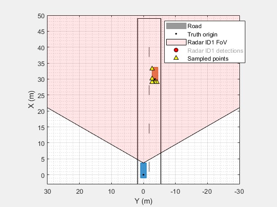
Use targetPoses (Automated Driving Toolbox) to generate detections from the straight road scenario that are exported using the Driving Scenario Designer (Automated Driving Toolbox) (DSD) app.
% Load the scenario and ego vehicle using the script exported from the DSD app
[scenario, egoVehicle] = helperStraightRoadDSDExport();
measLvlLRR.Profiles = actorProfiles(scenario); % Register the target profiles with the radar

% Get the target poses in the ego's body frame
tposes = targetPoses(egoVehicle);
time = scenario.SimulationTime;
dets = measLvlLRR(tposes,time);
Show the scenario ground truth and detections in a bird's-eye plot.
[bep,pltrs] = helperSetupDisplay(egoVehicle,measLvlLRR);
axis(bep.Parent,[-3 50 30*[-1 1]]);
pltrs.DetectionPlotters(1).Plotter(dets);

The generated detections lie along the outline of the target vehicle. Find the maximum signal-to-noise ratio (SNR) of the generated detections.
[measLvlSNR,iMax] = max(cellfun(@(d)d.ObjectAttributes{1}.SNR,dets(:)'));
disp(measLvlSNR)
67.2571
Compare the SNR of the detections generated by the measurement-level radar to the system-level radar in the Radar Designer app. The SNR exported by the Radar Designer app is the SNR for a single pulse (or sweep) of the radar. To compare the SNR predicted by the app to the measurement-level radar, the coherent processing gain from all pulses in the processing interval must be included.
% Use the exact range of the measurement. The measurement vector for this
% radar configuration is [az;rg;rr], so select the second element.
tgtRg = dets{iMax}.Measurement(2);
singleSweepSNR = interp1(target.ranges,availableSNR,tgtRg);
predictedSNR = singleSweepSNR + coherentIntGain
predictedSNR =
68.0891
ax = axes(figure);
X = categorical({'Predicted (Analytical Model)','Simulated (Meas-Level Model)'});
bar(ax,X,[predictedSNR measLvlSNR],'FaceColor', [0.75 1 0.75]);
xtickangle(ax,15)
grid(ax,'on')
ylabel(ax,'SNR (dB)')
title(ax,['SNR Verification: ' num2str(target.RCS) 'dBsm Target @ ' num2str(tgtRg,'%.1f') ' meters'])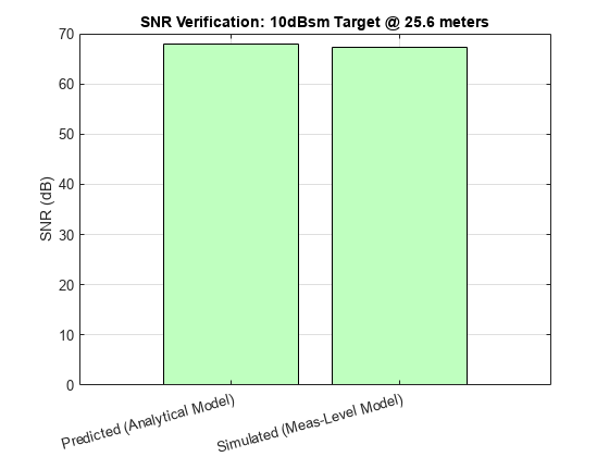
Create an Equivalent Radar Transceiver Model
Reuse the radarDataGenerator model to create an equivalent radarTransceiver that can simulate I/Q signals.
% Select the PRF based on the max radial speed constraint by setting the
% max unambiguous range accordingly
release(measLvlLRR);
lambda = lrrSysParam.Wavelength;
prfMaxSpeed = 4*speed2dop(predictedLRRMetrics{'First Blind Speed',end},lambda);
measLvlLRR.MaxUnambiguousRange = time2range(1/prfMaxSpeed,lambda*Fc);
xcvrLRR = radarTransceiver(measLvlLRR);
measLvlLRR.MaxUnambiguousRange = predictedLRRMetrics{'Unambiguous Range',end}; % Restore max range
disp(xcvrLRR)
  radarTransceiver with properties:

                Waveform: [1×1 phased.RectangularWaveform]
             Transmitter: [1×1 phased.Transmitter]
         TransmitAntenna: [1×1 phased.Radiator]
          ReceiveAntenna: [1×1 phased.Collector]
                Receiver: [1×1 phased.ReceiverPreamp]
      MechanicalScanMode: 'None'
      ElectronicScanMode: 'None'
        MountingLocation: [3.7000 0 0.2000]
          MountingAngles: [0 0 0]
    NumRepetitionsSource: 'Property'
          NumRepetitions: 256
       RangeLimitsSource: 'Property'
             RangeLimits: [0 3.8973e+03]
         RangeOutputPort: false
          TimeOutputPort: false
Model elaboration: antenna array design
The equivalent radarTransceiver has only a single element for transmit and for receive. A linear array is needed to measure azimuth. The number of array elements required to achieve the desired azimuth resolution is given by:
numElmnts = beamwidth2ap(measLvlLRR.AzimuthResolution,lambda,0.8859)*2/lambda % For an untapered arraynumElmnts = 72.5119
Use helperDesignArray to create the array configuration documented in [1] to realize the large array size required by the azimuth resolution.
[txArray, rxArray, arrayMetrics, txPos, rxPos, ant] = helperDesignArray(lambda,Fc);
Attach the designed transmit and receive antenna arrays to the radarTransceiver.
xcvrLRR.ReceiveAntenna.Sensor = rxArray;
xcvrLRR.TransmitAntenna.Sensor = txArray;
Set the electronic scan mode to 'Custom' and enable the weights input port on the transmit antenna to enable beamforming on transmit.
xcvrLRR.ElectronicScanMode = 'Custom';
xcvrLRR.TransmitAntenna.WeightsInputPort = true;
Model elaboration: waveform design
The radarTransceiver uses a rectangular waveform by default, but FMCW waveforms are more common in automotive radars. Attach an FMCW waveform to the radarTransceiver with its waveform parameters set to achieve the same range resolution as was used by the default rectangular waveform designed for the equivalent radar.
Fs = xcvrLRR.Waveform.SampleRate;
numSmps = ceil(Fs*lrrSysParam.Pulsewidth); % Must be a positive integer
wfm = phased.FMCWWaveform('SampleRate',Fs,'SweepTime',numSmps/Fs,'SweepBandwidth',Fs,'SweepInterval','Symmetric')
wfm =
  phased.FMCWWaveform with properties:

        SampleRate: 4.3000e+07
         SweepTime: 1.6907e-05
    SweepBandwidth: 4.3000e+07
    SweepDirection: 'Up'
     SweepInterval: 'Symmetric'
      OutputFormat: 'Sweeps'
         NumSweeps: 1
xcvrLRR.Waveform = wfm;
The sweep time computed for the radarTransceiver matches the sweep time of 17 us in Table 3 of [1].
Model elaboration: receiver noise figure and transmitted peak power
Adjust the transmitter's peak power level to account for the beamforming gains from the transmit and receive arrays and set the noise figure to match the value used by the design in the Radar Designer app.
Lnf = pow2db(radar.SystemTemperature/xcvrLRR.Receiver.ReferenceTemperature) % Noise figureLnf = 12.0000
xcvrLRR.Receiver.NoiseFigure = Lnf;
The power level computed for the transmitter agrees with the value of 13 dBm used in the Radar Designer app. A difference of 1 dB is explained by the rounded values taken from [1]-[3] that were entered in the app.
numReps = xcvrLRR.NumRepetitions;
xcvrLRR.NumRepetitions = lrrSysParam.NumCoherentPulses; % Use the number of repetitions specified in the app
pwr = (numReps/xcvrLRR.NumRepetitions)*xcvrLRR.Transmitter.PeakPower; % Keep the total power the same after changing the number of repetitions
pwrdBm = pow2db(pwr*1e3)-(arrayMetrics.TxGain+arrayMetrics.RxGain)-Lnf % dBm
pwrdBm =
14.1377
xcvrLRR.Transmitter.PeakPower = db2pow(pwrdBm)*1e-3; % WattsSimulate Radar Transceiver I/Q Signals
Create radar propagation paths from the target poses in the scenario. The extended target is modeled using a set of point targets located along the target's extent. The spacing of the point targets is determined by the azimuth and range resolution of the radar.
paths = poses2paths(tposes,xcvrLRR,scenario,measLvlLRR,bep);
Use radarTransceiver to generate baseband I/Q samples at the output of the radar receiver from the propagation paths for the target. The radar's field of view is electronically scanned by beamforming on transmit and stepping the transmit angle by the receive array's beamwidth.
azfov = measLvlLRR.FieldOfView(1);
numBeams = ceil(azfov/arrayMetrics.RxBeamwidth);
numBeams = floor(numBeams/2)*2+1; % Force the number of beams to be odd to keep a beam centered on 0 deg azimuth
azgrid = azfov*linspace(-0.5,0.5,numBeams);
Use phased.SteeringVector to compute steering vectors for the transmit array for each scan angle.
txSV = phased.SteeringVector( ...
    'SensorArray',xcvrLRR.TransmitAntenna.Sensor, ...
    'PropagationSpeed',xcvrLRR.TransmitAntenna.PropagationSpeed);
txSteer = txSV(xcvrLRR.TransmitAntenna.OperatingFrequency,azgrid);
Use radarTransceiver to collect baseband I/Q datacubes for each scan angle.
numFT = xcvrLRR.Waveform.SampleRate*xcvrLRR.Waveform.SweepTime; % Number of fast-time samples (range bins)
numST = xcvrLRR.NumRepetitions; % Number of slow-time samples (Doppler bins)
numRxElmnts = getNumElements(xcvrLRR.ReceiveAntenna.Sensor); % Number of receive array elements
numFrames = numel(azgrid); % Number of frames (scan angles)

% Allocate array to collect datacubes
Xframes = NaN(numFT,numRxElmnts,numST,numFrames);

% Advance the simulation time by the duration of each frame
tFrame = xcvrLRR.Waveform.SweepTime*xcvrLRR.NumRepetitions;
for iFrm = 1:numFrames
    % Current scan angle
    txAng = [azgrid(iFrm);0];

    % Collect datacube at current scan angle
    Xcube = xcvrLRR(paths,time+(iFrm-1)*tFrame,conj(txSteer(:,iFrm)));
    Xframes(:,:,:,iFrm) = Xcube;
end
Show the spectrogram of the collected datacube for a scan angle in the direction of the target.
% Find the scan angle closest to the target's direction
tgtAng = [paths.AngleOfArrival];
tgtAz = mean(tgtAng(1,:));
[~,iFrm] = min(abs(azgrid-tgtAz));

% Show the spectrogram for the data taken from the first sweep and first
% receive element
ax = axes(figure);
spectrogram(Xframes(:,1,1,iFrm),[],[],[],Fs);
title(ax,'FMCW Return from Target')
clim(ax,'auto')
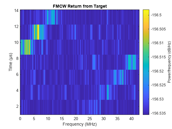
drawnow
Process I/Q Signals into Object Detections
Apply range, Doppler, and beamform processing
Use helperRangeDopplerProcessing to apply range and Doppler processing for each frame of the I/Q data.
[Xrngdop,rggrid,rrgrid] = helperRangeDopplerProcessing(Xframes,xcvrLRR);
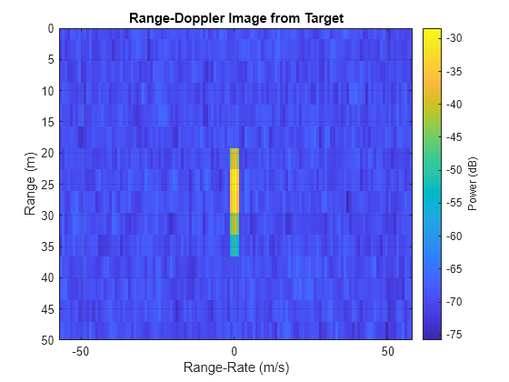
Show the range-Doppler image for the scan angle in the direction of the target.
Xdb = pow2db(abs(Xrngdop).^2);

% Select the frame with the largest return, that is probably the target
[~,iMax] = max(Xdb(:));
[~,~,~,iFrm] = ind2sub(size(Xdb),iMax);
ax = axes(figure);
imagesc(ax,rrgrid,rggrid,squeeze(max(Xdb(:,:,:,iFrm),[],2))); % Select the max across the receive elements
xlabel(ax,'Range-Rate (m/s)'); ylabel(ax,'Range (m)');
set(ax,'YDir','reverse'); ylim(ax,[0 50]); grid(ax,'on');
title(ax,'Range-Doppler Image from Target');
set(get(colorbar(ax),'YLabel'),'String','Power (dB)');
Use helperBeamProcessing to apply beamforming for the virtual array at each scan direction.
Xbmfrngdop = helperBeamProcessing(Xrngdop,xcvrLRR,azgrid);
The returned datacube has dimensions: range x azimuth x Doppler.
disp(size(Xbmfrngdop))
364 91 128
Generate and cluster detections
Use helperFindDetections to compare the SNR of the range, Doppler, and beamformed datacube to a detection threshold. Select the detection threshold to match the desired detection probability of 0.9 and false alarm rate of 1e-6 of our initial radar design.
Pd = predictedLRRMetrics{'Probability of Detection',3}Pd = 0.9000
Pf = lrrSysParam.Pfa
Pf =
1.0000e-06
[iDet,estnoiselvldB,threshdB] = helperFindDetections(Xbmfrngdop,Xrngdop,xcvrLRR,Pd,Pf);
Show the number of detections found in the processed radar data.
numel(iDet)
ans =
17
There are more detected threshold crossings than there are targets. Multiple threshold crossings are expected for each detected target. This occurs not only for extended targets, but even in the case of point targets. This is because the ambiguity functions associated with the waveform and array are not an impulse response but have a sinc-type shape. As a result, multiple range, Doppler, and beam bins may cross the threshold level for a single point target. This is especially true for targets that have a large signal-to-noise ratio (SNR), such as those with a large RCS or that are very close to the radar. Detection crossings need to be clustered to address this. DBSCAN is a common algorithm used for this. Use the clusterDBSCAN to identify threshold crossings that are likely coming from a single target. Use helperIdentifyClusters to identify clusters of detections.
[clusterIDs,detidx,numClusters] = helperIdentifyClusters(Xbmfrngdop,iDet,azgrid,rggrid,rrgrid);
disp(numClusters)
5
The number of clustered detections now agrees with the number of point targets used to model the extended target.
Estimate range, range-rate, and azimuth for each cluster
Use helperMeasurementEstimation to estimate the range, range-rate, and azimuth angle associated with each cluster of detection threshold crossings.
[meas,noise,snrdB] = helperMeasurementEstimation(Xbmfrngdop,estnoiselvldB,xcvrLRR,azgrid,rggrid,rrgrid,clusterIDs,detidx);
Use helperAssembleDetections to assemble the detections into a cell array of objectDetection objects. This is the interface used by the trackers that ship with Radar toolbox and Sensor Fusion and Tracking toolbox. This also matches the format returned by radarDataGenerator.
dets = helperAssembleDetections(xcvrLRR,time,meas,noise,snrdB)
dets=5×1 cell array
    {1×1 objectDetection}
    {1×1 objectDetection}
    {1×1 objectDetection}
    {1×1 objectDetection}
    {1×1 objectDetection}
Plot the range-angle image of the SNR values in the range, Doppler, and beamformed datacube and overlay the image with the signal-level detections extracted from the datacube.
axRgAz = helperPlotRangeAzimuthDetections(bep,Xbmfrngdop,estnoiselvldB,threshdB,xcvrLRR,azgrid,rggrid,dets);

Compare Simulated Measurements with Predicted Metrics
Find the maximum SNR from the signal-level detections.
sigLvlSNR = max(cellfun(@(d)d.ObjectAttributes{1}.SNR,dets(:)'));Include processing loss from the target's range relative to the duration of the FMCW sweep. This loss can be reduced by increasing the sweep time of the FMCW waveform, but with the cost of processing more data and longer waveform transmission times.
Lsweep = pow2db(numel(rggrid)/sum(rggrid<tgtRg)) % Loss due to range of target and FMCW sweep durationLsweep = 16.5801
sigLvlSNR = sigLvlSNR+Lsweep;
Compare the SNR of the detections generated by the signal-level radar to the measurement-level and system-level radars. after accounting for the sweep loss.
ax = axes(figure);
X = categorical({'Predicted (Analytical Model)','Simulated (Meas-Level Model)','Simulated (Signal-Level Model)'});
bar(ax,X,[predictedSNR measLvlSNR sigLvlSNR],'FaceColor', [0.75 1 0.75]);
xtickangle(ax,15)
grid(ax,'on')
ylabel(ax,'SNR (dB)')
title(ax,['SNR Verification: ' num2str(target.RCS) 'dBsm Target @ ' num2str(tgtRg,'%.1f') ' meters'])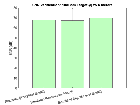
The detections generated from radarTransceiver agree with the system- and measurement-level models. A small variation, less-than 3 dB, in SNR is expected due to losses present in the signal-level model that are not included or are assumed constant in the measurement- and system-level models.
Compare the detection locations between the signal-level and measurement-level radars.
plotSideBySide(axRgAz,bep);
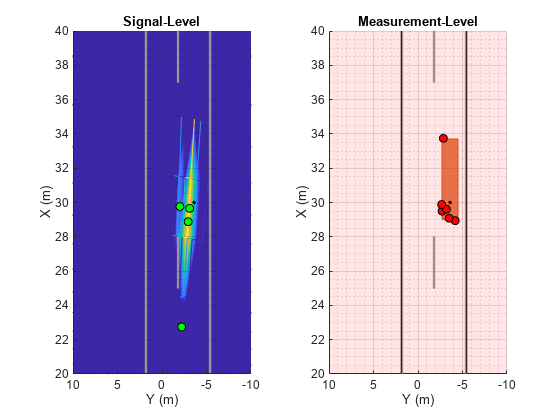
Both radar models generate detections that lie along the exterior of the extended target.
Summary
In this example, you learned how to design and predict performance for a system-level radar using the Radar Designer app. You then learned how to create an equivalent measurement-level radar from the system-level design by using radarDataGenerator to generate consistent SNR for the generated detections. You then learned how to generate an equivalent signal-level radar using radarTransceiver. You simulated I/Q data using radarTransceiver and applied range, Doppler, and beamforming to the I/Q data to extract detections for the baseband I/Q radar data. The signal-level detections were consistent with the measurement-level and system-level radar models and satisfied the design requirements of the original system-level radar.
References
[1] Texas Instruments Incorporated, "Design Guide: TIDEP-01012 - Imaging Radar Using Cascaded mmWave Sensor Reference Design," Texas Instruments, Post Office Box 655303, Dallas, Mar 2020.
[2] Texas Instruments Incorporated, "AWR2243 Single-Chip 76- to 81-GHz FMCW Transceiver," Texas Instruments, Post Office Box 655303, Dallas, Aug 2020.
[3] Texas Instruments Incorporated, "User's Guide: AWRx Cascaded Radar RF Evaluation Module - (MMWCAS-RF-EVM)," Texas Instruments, Post Office Box 655303, Dallas, Feb 2020.
Helper Functions
helperDesignArray
Use helperDesignArray to create the array configuration documented in [1] to realize the large array size required by the azimuth resolution.
[txArray, rxArray, arrayMetrics, txPos, rxPos, ant] = helperDesignArray(lambda,Fc);
Confirm that the directivity of the phased.CosineAntennaElement matches the directivity of 12 dBi reported in Table 1 of [3]. Directivity is strongly related to an antenna's field of view.
disp(pattern(ant,Fc,0,0))
12.6731
Confirm that the receive array gain matches the gain of 24 dBi modeled in the Radar Designer app.
Grx = pattern(rxArray,Fc,0,0)
Grx =
23.5432
Compute the azimuth 3-dB beamwidth for the receive array. The 3-dB beamwidth should match the desired azimuth resolution of 1.4 degrees.
rxAzBw = beamwidth(rxArray,Fc,'Cut','Azimuth')
rxAzBw =
1.3400
Confirm that the transmit array gain matches the gain of 23 dBi modeled in the Radar Designer app.
Gtx = pattern(txArray,Fc,0,0)
Gtx =
23.3902
The transmit array beamwidth is larger than the receive array beamwidth. This is useful since the look directions will be spaced according to the radar's azimuth resolution. The larger transmit beamwidth ensures that all targets within a receive beamwidth will be illuminated by the transmit beam.
txAzBw = beamwidth(txArray,Fc,'Cut','Azimuth')
txAzBw =
3.1800
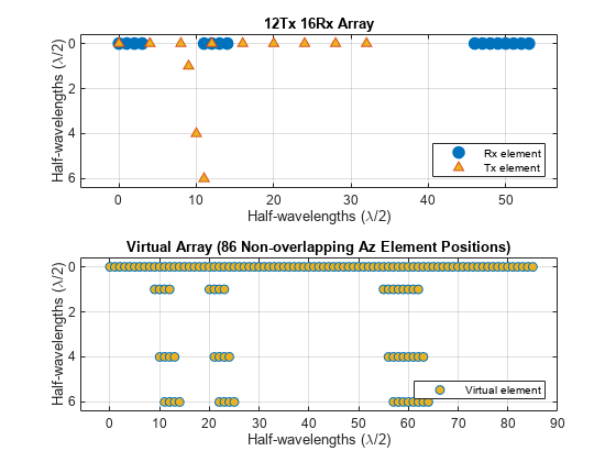
Compute the virtual array element positions by convolving the transmit and receive array element positions. Plot the receive, transmit, and virtual array element positions. The resulting array is a 2D array with the x-axis corresponding to the horizontal elements used to measure azimuth and the y-axis corresponds to vertical elements.
vxPos = conv2(txPos,rxPos);
viewArray(txArray,rxArray,lambda,vxPos)
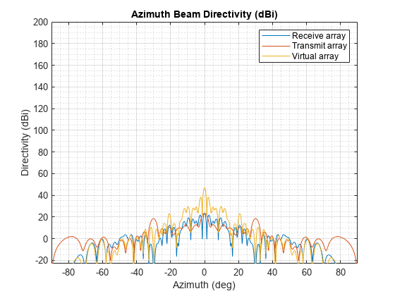
Plot the directivity of the transmit, receive, and virtual arrays.
plotDirectivities(txArray,rxArray,Fc)
helperRangeDopplerProcessing
helperRangeDopplerProcessing creates a phased.RangeDopplerResponse and uses helperRangeDopplerProcess to apply range and Doppler processing to the collected datacubes.
[Xrngdop,rggrid,rrgrid,rngdopproc] = helperRangeDopplerProcessing(Xframes,xcvrLLR)
By default, Hanning windows are used in range and Doppler to suppress sidelobes in these dimensions.
rngWinFcn = @hanning;
dopWinFcn = @hanning;

rngdopproc = phased.RangeDopplerResponse('RangeMethod','FFT', ...
    'DopplerOutput','Speed','SweepSlope',xcvrLRR.Waveform.SweepBandwidth/xcvrLRR.Waveform.SweepTime);

% Configure Doppler properties
rngdopproc.PropagationSpeed = xcvrLRR.ReceiveAntenna.PropagationSpeed;
rngdopproc.OperatingFrequency = xcvrLRR.ReceiveAntenna.OperatingFrequency;
rngdopproc.SampleRate = xcvrLRR.Receiver.SampleRate;
rngdopproc.DopplerWindow = 'Custom';
rngdopproc.CustomDopplerWindow = dopWinFcn;
rngdopproc.DopplerFFTLengthSource = 'Property';
Nd = 2^nextpow2(xcvrLRR.NumRepetitions);
rngdopproc.DopplerFFTLength = Nd;

% Release memory
clear Xrngdop rggrid rrgrid

[Xrngdop,rggrid,rrgrid] = helperRangeDopplerProcess(rngdopproc,Xframes,xcvrLRR,rngWinFcn);
helperBeamProcessing
helperBeamProcessing processes the receive beams for each of the scan angles.
Xbmfrngdop = helperBeamProcessing(Xrngdop,xcvrLLR,azgrid);
helperBeamProcessing uses phased.SteeringVector to compute the steering vectors for the receive array and helperVirtualBeamform to compute the steering vectors for the virtual array and beamform at each scan angle. Use a Hanning window across the non-overlapping elements of the virtual array to suppress azimuth sidelobes.
bmfWinFcn = @hanning;

rxSV = phased.SteeringVector( ...
    'SensorArray',xcvrLRR.ReceiveAntenna.Sensor, ...
    'PropagationSpeed',xcvrLRR.ReceiveAntenna.PropagationSpeed);
rxSteer = rxSV(xcvrLRR.ReceiveAntenna.OperatingFrequency,azgrid);

Xbmfrngdop = helperVirtualBeamform(txSteer,rxSteer,Xrngdop,bmfWinFcn);
helperFindDetections
helperFindDetections extracts detection locations in the range-Doppler and beamform processed datacube.
Compare the SNR of the range, Doppler, and beamformed datacube to a detection threshold. Select the detection threshold to match the desired detection probability of 0.9 and false alarm rate of 1e-6 of our initial radar design.
Pd = predictedLRRMetrics{'Probability of Detection',3};
Pf = lrrSysParam.Pfa;

threshdB = detectability(Pd,Pf)
threshdB = 13.1217
Compute the SNR of the processed radar datacube. First, estimate the noise floor of the processed data by collecting noise only data. This is noise only data is often collected between transmissions during the idle time of the transceiver or between repetition intervals. A CFAR estimator such as phased.CFARDetector2D could also be used to estimate the noise level in cases where the noise floor is not constant.
noSignal = zeros(numFT,numRxElmnts,numST);
Ncube = xcvrLRR.Receiver(noSignal(:));
Ncube = reshape(Ncube,numFT,numRxElmnts,numST);
Apply the same range, Doppler, and beamform processing to the noise data as was applied to the detection data.
Nrngdop = helperRangeDopplerProcess(rngdopproc,Ncube,xcvrLRR,rngWinFcn);
Nbmfrngdop = helperBeamProcessing(Nrngdop,xcvrLRR,0,bmfWinFcn);

% Estimate noise level in dB
estnoiselvldB = pow2db(mean(abs(Nbmfrngdop(:)).^2))
estnoiselvldB = -51.3781
Normalize the radar datacube using the noise floor estimate.
Xpow = abs(Xbmfrngdop).^2; % Power is amplitude squared
XsnrdB = pow2db(Xpow)-estnoiselvldB; % Normalize using the estimated noise floor power level to get SNR
clear Xpow % release memory
Compare the SNR values in the radar datacube to the detection threshold to identify range, Doppler, and azimuth resolution cells that have detections.
isDet = XsnrdB(:)>threshdB;

% Number of detection threshold crossings
sum(isDet)
ans = 516
Many of the threshold crossings correspond to the sidelobes of the virtual array. Suppression of the sidelobes using a spatial taper alone is often not enough to avoid these spurious detections. Identify sidelobe detections by comparing the SNR of the detection locations for a single element to the SNR in the beams.
% Estimate sidelobe level from sidelobe detections
estnoiseslldB = pow2db(mean(abs(Nrngdop(:)).^2));

XslldB = squeeze(max(pow2db(abs(Xrngdop).^2),[],2)); % Max across receive elements
XslldB = XslldB-estnoiseslldB; % Convert to SNR
XslldB = permute(XslldB,[1 3 2]); % range x azimuth x Doppler
isLob = isDet & XsnrdB(:)<XslldB(:);
sum(isLob)
ans =
391
Adjust the detection threshold according to the max sidelobe level to further suppress sidelobe detections.
maxSLLdB = max(XslldB(isLob)-XsnrdB(isLob))
maxSLLdB =
29.0486
clear XslldB % release memory
threshdB = threshdB+maxSLLdB
threshdB =
42.1703
iDet = find(XsnrdB(:)>threshdB & ~isLob);
Remaining number of detections after removal of sidelobe threshold crossings.
numel(iDet)
ans =
10
helperIdentifyClusters
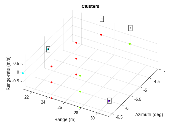
helperIdentifyClusters identifies groups of detection locations coming from a common target. The returned list of cluster IDs are used for measurement estimation from each cluster of detections.
There are more detected threshold crossings than there are targets. Multiple threshold crossings are expected for each detected target. This occurs not only for extended targets, but even in the case of point targets. This is because the ambiguity functions associated with the waveform and array are not an impulse response but have a sinc-type shape. As a result, multiple range, Doppler, and beam bins may cross the threshold level for a single point target. This is especially true for targets that have a large signal-to-noise ratio (SNR), such as those with a large RCS or that are very close to the radar. Detection crossings need to be clustered to address this. DBSCAN is a common algorithm used for this. Use the clusterDBSCAN to identify threshold crossings that are likely coming from a single target.
% Compute the range, angle, and Doppler indices of the detection crossings
[iRg,iAng,iRr] = ind2sub(size(XsnrdB),iDet);
detidx = [iRg iAng iRr];

% Select the range, angle, and Doppler bin centers associated with each
% detection crossing
meas = [rggrid(iRg) azgrid(iAng)' rrgrid(iRr)];
Estimate the epsilon to use for DBSCAN clustering.
minNumPoints = 2;
maxNumPoints = 10;
epsilon = clusterDBSCAN.estimateEpsilon(meas,minNumPoints,maxNumPoints)
epsilon =
2.9206
% Range and Doppler ambiguity limits
ambLims = [ ...
    [min(rggrid) max(rggrid)]; ...
    [min(rrgrid) max(rrgrid)]];
clusterDets = clusterDBSCAN( ...
    'MinNumPoints',1, ...
    'EnableDisambiguation',true, ...
    'AmbiguousDimension',[1 3], ...
    'Epsilon',epsilon);
Identify the detections that should be clustered into a single detection. The threshold crossings are assigned IDs. Crossings that appear to come from the same target will be assigned the same ID.
[indClstr,clusterIDs] = clusterDets(meas,ambLims);
clusterIDs = clusterIDs(:)';

% Number of unique targets estimated after clustering the threshold crossings.
if isempty(clusterIDs)
    numDets = 0;
else
    numDets = max(clusterIDs);
end

% Plot clusters
ax = axes(figure);
plot(clusterDets,meas,indClstr,'Parent',ax);
xlabel(ax,'Range (m)'); ylabel(ax,'Azimuth (deg)'); zlabel(ax,'Range-rate (m/s)');
view(ax,[30 60]);
viewArray
viewArray displays the element positions of the transmit, receive, and virtual arrays generated by helperDesignArray.
function viewArray(txArray,rxArray,lambda,vxPos)
tl = tiledlayout(figure,2,1,'TileSpacing','loose');

% Plot Tx an Rx arrays
ax = nexttile(tl);
clrs = colororder(ax);
spacing = lambda/2;
p1 = plot(ax,rxArray.ElementPosition(2,:)/spacing,rxArray.ElementPosition(3,:)/spacing,'o','MarkerSize',8,'MarkerFaceColor',clrs(1,:));
hold(ax,'on'); drawnow;
p2 = plot(ax,txArray.ElementPosition(2,:)/spacing,txArray.ElementPosition(3,:)/spacing,'^','MarkerFaceColor',clrs(3,:));
xlabel(ax,'Half-wavelengths (\lambda/2)'); ylabel(ax,'Half-wavelengths (\lambda/2)');
title(ax,'12Tx 16Rx Array'); grid(ax,'on');
set(ax,'YDir','reverse');
legend([p1 p2],'Rx element','Tx element','Location','SouthEast');
xlim(ax,'padded'); ylim(ax,'padded');

% Plot virtual array
ax = nexttile(tl);
[row,col] = ind2sub(size(vxPos),find(vxPos(:)));
p3 = plot(ax,row-1,col-1,'o','Color',clrs(1,:),'MarkerFaceColor',clrs(3,:));
xlabel(ax,'Half-wavelengths (\lambda/2)'); ylabel(ax,'Half-wavelengths (\lambda/2)');
title(ax,'Virtual Array (86 Non-overlapping Az Element Positions)'); grid(ax,'on');
set(ax,'YDir','reverse');
legend(p3,'Virtual element','Location','SouthEast');
xlim(ax,'padded'); ylim(ax,'padded');
end
plotDirectivities
plotDirectivities plots the azimuth antenna patterns for the transmit, receive, and virtual arrays.
function plotDirectivities(txArray,rxArray,Fc)
angs = -180:0.1:180;
patRx = patternAzimuth(rxArray,Fc,'Azimuth',angs);
patTx = patternAzimuth(txArray,Fc,'Azimuth',angs);
patVx = patTx+patRx;

ax = axes(figure);
p1 = plot(ax,angs,patRx);
hold(ax,'on');
p2 = plot(ax,angs,patTx);
p3 = plot(ax,angs,patVx);
xlabel(ax,'Azimuth (deg)'); ylabel(ax,'Directivity (dBi)');
Gmax = max([patRx(:);patTx(:);patVx(:)]);
grid(ax,'on'); grid(ax,'minor');
ylim(ax,[Gmax-70 max(ylim)]); xlim(ax,[-90 90]);
title(ax,'Azimuth Beam Directivity (dBi)');
legend([p1 p2 p3],'Receive array','Transmit array','Virtual array');
end
poses2paths
poses2paths converts the target poses to a path struct array defining the two-way freespace propagation paths between the radarTransceiver and the targets in the scenario.
function paths = poses2paths(tposes,txrx,scenario,rdr,bep)
% Transport the target poses from the ego's body frame to the sensor's
% mounted frame
tposesMnt = helperPosesToSensorFrame(tposes,txrx);

% Sample target extent and compute RCS and viewed angles
rf = txrx.ReceiveAntenna.OperatingFrequency;
lambda = freq2wavelen(rf,txrx.ReceiveAntenna.PropagationSpeed);

% Profiles define the dimensions and RCS of the targets
profiles = actorProfiles(scenario);

% Compute the angle at which each target is viewed by the sensor
[rcsdBsm,tids] = helperTargetRCS(tposesMnt,profiles,rf);

map = containers.Map(tids,rcsdBsm);
rcsTbl = @(ids)arrayfun(@(id)map(id),ids); % Create a lookup table

% Map the targets to sets of points according to the sensor's resolution
res = NaN(1,3);
res(1) = rdr.AzimuthResolution;
if rdr.HasElevation
    res(2) = rdr.ElevationResolution;
end
res(3) = rdr.RangeResolution;
rgLim = [0 rdr.RangeLimits(2)];
fov = rdr.FieldOfView;
[posMnt,velMnt,ids] = helperSphericallySampleTargets(tposesMnt,profiles,res,fov,rgLim);
rcsdBsm = rcsTbl(ids);

[rot,off] = helperSensorFrame(txrx);
posBdy = rot*posMnt + off;

if nargin>4
    % Hide the detections
    h = findobj(bep.Parent,'Tag','bepTrackPositions_Radar ID1 detections');
    h.Visible = 'off';
    %clearData(bep.Plotters(end)); % Clear detections

    hold(bep.Parent,'on');
    hndl = plot(bep.Parent,posBdy(1,:),posBdy(2,:),'^k','MarkerFaceColor','y','DisplayName','Sampled points');
    hold(bep.Parent,'off');
    leg = legend(bep.Parent);
    leg.PlotChildren = [leg.PlotChildren;hndl];
end

paths = helperFreespacePaths(posMnt,velMnt,lambda,rcsdBsm);
end
plotSideBySide
plotSideBySide creates a side-by-side comparison of the detections generated using radarTransceiver on the left and the detections generated using radarDataGeneartor on the right.
function plotSideBySide(axRgAz,bep)
tl = tiledlayout(figure,1,2,'TileSpacing','loose');

ax = nexttile(tl);
copyobj(axRgAz.Children,ax);
view(ax,-90,90)
axis(ax,axis(axRgAz));
clim(ax,clim(axRgAz));
xlabel(ax,'X (m)'); ylabel(ax,'Y (m)');
title(ax,'Signal-Level');
grid(ax,'on'); grid(ax,'minor');
set(ax,'Layer','top');
ylim(ax,10*[-1 1])

ax = nexttile(tl);
axBEP = bep.Parent;
shh = get(groot,'ShowHiddenHandles');
set(groot,'ShowHiddenHandles','on');
copyobj(axBEP.Children,ax);
set(groot,'ShowHiddenHandles',shh);
view(ax,-90,90)

axis(ax,axis(axRgAz));
xlabel(ax,'X (m)'); ylabel(ax,'Y (m)');
title(ax,'Measurement-Level');
grid(ax,'on'); grid(ax,'minor');
ylim(ax,10*[-1 1])

h = findobj(ax,'Tag','bepTrackPositions_Radar ID1 detections');
if ~isempty(h) && ishghandle(h)
    h.Visible = 'on';
end

h = findobj(ax,'DisplayName','Sampled points');
if ~isempty(h) && ishghandle(h)
    delete(h);
end
end