Radar Designer

Model radar gains and losses and assess performance in different environments

Since R2021a

Description

The Radar Designer app is an interactive tool that assists engineers and system analysts with high-level design and assessment of conventional air and ground-based radar systems at the early stage of radar development. Using the app, you can:

• Assess and compare multiple radar designs in a single session

• Add smart radar, environment, and target Radar Designer Configurations to jump-start your analysis

• Incorporate environmental effects due to Earth's curvature, atmosphere, terrain, and precipitation

• Add custom target radar cross-sections, antenna/array models, and both range-independent and range-dependent losses

• Export and save results, sessions, models, and plots to continue your analysis

• Export a MATLAB^® script to simulate the radar detecting a target in a dynamic scenario (since R2024b)

Open the Radar Designer App

• MATLAB Toolstrip: On the Apps tab, under Signal Processing and Communications, click the app icon.

• MATLAB command prompt: Enter radarDesigner.

Examples

Design Automotive Radar

Design a radar to install on top of a truck. Adjust the design parameters so the radar can work in foggy conditions and still make the objective range. Export the design session to the MATLAB Workspace.

Open Radar Designer. At the command line, type

radarDesigner

Start a radar design session. On the toolstrip, click New Session and select the Automotive Radar option. The app specifies typical automotive radar design, target, and environment parameters.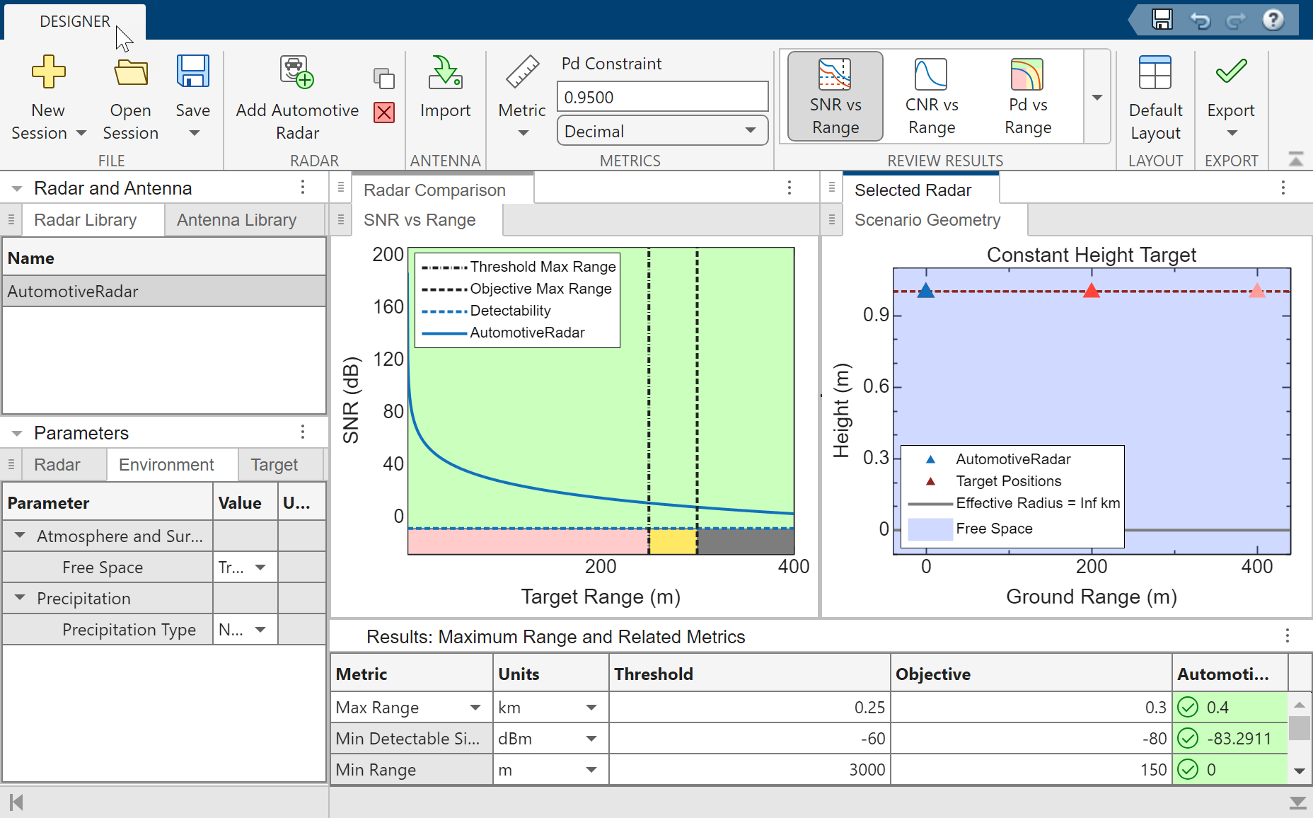

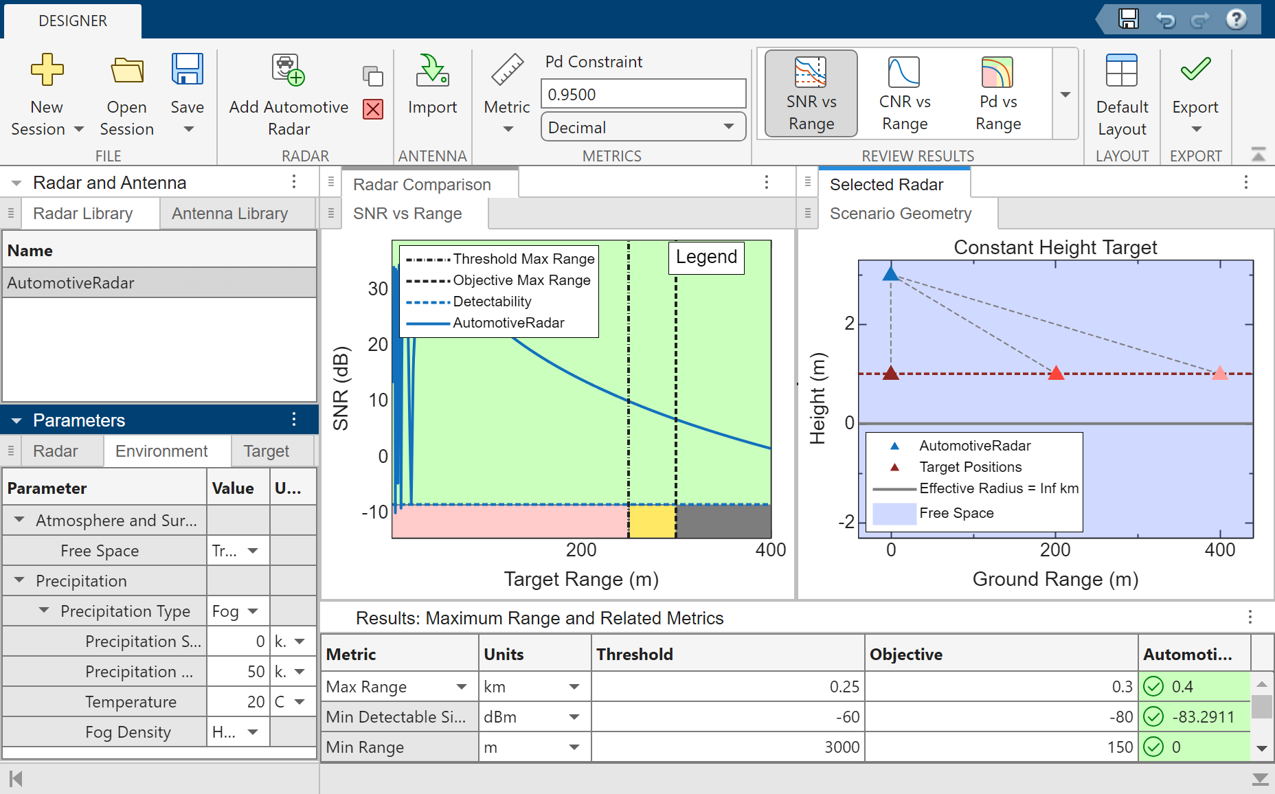
The radar you are designing must be set 3 meters above the ground. On the Radar tab, in the Antenna and Scanning section, change the Antenna Height from 1 meter to 3 meters.

On the Environment tab, in the Precipitation section, specify the Precipitation Type as Fog and set the Fog Density to Heavy.

As the SNR vs Range plot and Metrics and Requirements table show, the radar satisfies the threshold maximum range but falls short of the desired maximum range of 300 meters.

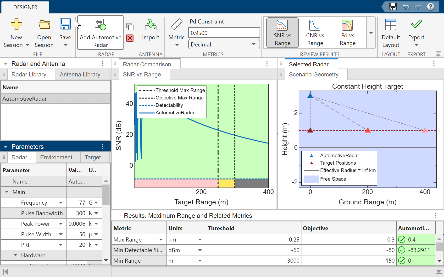
Increase the transmitted power to attain a higher maximum range. On the Radar tab, in the Main section, increase the Peak Power to 6e-04 kW. The plot and table show that the radar satisfies the requirement with the new power value.

Export the radar design to the MATLAB Workspace. On the toolstrip, click Export and select Generate Metrics Report to generate a formatted report of numeric metrics.

Related Examples

• Radar Link Budget Analysis
• Radar Design Part I: From Power Budget Analysis to Dynamic Scenario Simulation
• Radar Design Part II: From Radar Data to IQ Signal Synthesis

Parameters

Radar and Antenna

Radar Library — Radar library selection table

tab

Select the current radar from the Radar Library tab of the Radar and Antenna table. To populate this table, click New Session on the app toolstrip to load one of the built-in Radar Designer Configurations. Use the Add Radar toolstrip button to add additional radars. Select the current radar from the Name list or rename a radar design. Switch between the listed radars to quickly assess and compare design viability.

Antenna Library — Antenna library selection table

tab

Since R2025a

Use the Import Antenna toolstrip button to import antennas into the Antenna Library tab of the Radar and Antenna table. A default antenna, DefaultSinc, is automatically listed. Nonpolarized Phased Array System Toolbox™ antenna objects are supported. Antennas from the antenna library can be selected in the Antenna and Scanning menu of the Radar parameter tab.

Radar, Target, and Environment

Radar — Design parameters

tab

Use the Radar section of the app toolstrip to change

Main — Pulse and carrier settings

tab section

Use these parameters to specify pulse and carrier settings, such as the carrier frequency and the transmitted power.

Parameter	Description
Frequency (default) or Wavelength	Carrier frequency or carrier wavelength, specified as a scalar. Specify Frequency as a scalar in Hz, kHz, MHz, or GHz. Specify Wavelength as a scalar in m, cm, or mm.
Pulse Bandwidth	Bandwidth of the transmitted pulse, specified as a scalar in Hz, kHz, MHz, or GHz.
Peak Power (default) or Average Power	Average transmitted power or peak transmitted power, specified as a scalar. Specify Peak Power as a scalar in W, kW, MW, dBW, or dBm. Specify Average Power as a scalar in W, kW, MW, dBW, or dBm.
Pulse Width (default) or Duty Cycle	Radar pulse width or radar duty cycle, specified as a scalar. Specify Pulse Width, the duration of the transmitted pulse, as a scalar in s, ms, or μs. Specify Duty Cycle, fraction of the time the radar is transmitting, as a dimensionless scalar from 0 to 1.
PRF (default) or PRI	Pulse repetition frequency (PRF) or pulse repetition interval (PRI), specified as a scalar. Specify PRF, the number of pulses transmitted per second, as a scalar in Hz, kHz, or MHz. Specify PRI, the time between two consecutive transmitted pulses, as a scalar in s, ms, or μs.

Hardware — Noise settings

tab subsection

Use these parameters to specify noise settings, such as noise temperature or dynamic range.

Parameter	Description
Noise Temperature or Noise Figure	System noise temperature or noise figure, specified as a scalar. Specify Noise Temperature as a scalar in K. Specify Noise Figure as a scalar in dB or in linear units.
Reference Noise Temperature	Reference noise temperature, specified as a scalar in K.
Quantization Noise	Select Ignored (default) to ignore quantization noise or Included to include quantization noise.
Number of Bits	Number of bits in the analog-to-digital (A/D) converter, specified as a dimensionless scalar. This parameter applies only if Quantization Noise is included.
Dynamic Range	Dynamic range of the A/D converter, specified as a scalar in dB or in linear units. This parameter applies only if Quantization Noise is included.

Antenna and Scanning — Position, beamwidth, and gain settings

tab section

Use these parameters to specify antenna pattern, position, beamwidth, and gain settings, such as antenna height, antenna polarization, or azimuth beamwidth.

Parameter	Description
Antenna Height	Height of the antenna above the surface, specified as a scalar in m, km, ft, or kft. This parameter applies to both the transmit antenna and the receive antenna.
Antenna Tilt Angle	Angle between the electric axis of the antenna and the ground plane, specified as a scalar in deg, rad, or mrad. This parameter applies to both the transmit antenna and the receive antenna.
Antenna Polarization	Specify the antenna polarization as Horizontal or Vertical. This parameter applies to both the transmit antenna and the receive antenna.

Transmit Antenna — Transmit antenna

tab subsection

Specify the Transmit Antenna as Sinc Antenna Pattern or select an Antenna Library antenna:

• Sinc Antenna Pattern — Uses a sinc antenna pattern. Specify the Gain manually or automatically calculate the Gain by specifying the Azimuth Beamwidth, and Elevation Beamwidth, assuming an ideal Gaussian beam pattern. Note that the automatically calculated Gaussian gain is different from the gain that is automatically populated for the DefaultSinc Antenna Library antenna, which does not assume a Gaussian beam pattern.

  Parameter	Description
  Sinc Gain Input	Select either Manual Gain or From Beamwidth Manual Gain — Use the Gain box to enter a custom value for the transmit antenna in dBi. From Beamwidth — Compute the transmit antenna gain from the beamwidths assuming an ideal Gaussian beam pattern with no sidelobes. The resulting gain is displayed in the Gain box.
  Azimuth Beamwidth	Azimuth beamwidth of the transmit antenna, specified as a scalar in deg, rad, or mrad. This parameter applies only if From Beamwidth is selected under Sinc Gain Input.
  Elevation Beamwidth	Elevation beamwidth of the transmit antenna, specified as a scalar in deg, rad, or mrad. This parameter applies only if From Beamwidth is selected under Sinc Gain Input.

• Antenna Library — Select an antenna from the Antenna Library. The name of the selected antenna is displayed in the Imported Antenna Object box. The Azimuth Beamwidth, Elevation Beamwidth, and Gain for the transmit antenna pattern are automatically populated.

Use Different Antenna for Receive — Receive antenna

tab subsection

Select Use Different Antenna for Receive to indicate that the receive and transmit antennas have different gains or select a distinct antenna pattern from the Antenna Library. If you select True to use a different antenna for receive, you can specify the Receive Antenna as Sinc Antenna Pattern or select an Antenna Library antenna:

• Sinc Antenna Pattern — Uses a sinc antenna pattern. Specify the Gain manually or automatically calculate the Gain by specifying the Azimuth Beamwidth, and Elevation Beamwidth, assuming an ideal Gaussian beam pattern. Note that the automatically calculated Gaussian gain is different from the gain that is automatically populated for the DefaultSinc Antenna Library antenna, which does not assume a Gaussian beam pattern.

  Parameter	Description
  Sinc Gain Input	Select either Manual Gain or From Beamwidth Manual Gain — Use the Gain box to enter a custom value for the receive antenna in dBi. From Beamwidth — Compute the receive antenna gain from the beamwidths assuming an ideal Gaussian beam pattern with no sidelobes. The resulting gain is displayed in the Gain box.
  Azimuth Beamwidth	Azimuth beamwidth of the transmit antenna, specified as a scalar in deg, rad, or mrad. This parameter applies only if From Beamwidth is selected under Sinc Gain Input.
  Elevation Beamwidth	Elevation beamwidth of the transmit antenna, specified as a scalar in deg, rad, or mrad. This parameter applies only if From Beamwidth is selected under Sinc Gain Input.

• Antenna Library — Select an antenna from the Antenna Library. The name of the selected antenna is displayed in the Imported Antenna Object box. The Azimuth Beamwidth, Elevation Beamwidth, and Gain for the receive antenna pattern are automatically populated.

Scan Mode — Scan mode settings

tab subsection

Specify the scan mode for your design as one of these:

• None — The radar performs no scanning. Radar Designer does not incorporate scanning-related losses into the analysis.

• Mechanical — The radar performs mechanical scanning. Radar Designer incorporates beam shape loss and beam-dwell factor (range-dependent loss for rapidly scanning beam) into the analysis.

• Electronic — The radar uses a phased array to perform electronic scanning. Radar Designer incorporates beam shape loss and scan sector loss into the analysis.

If you specify Scan Mode as Mechanical or Electronic, you can set these parameters.

Parameter	Description
Azimuth Scan Sector Size	Azimuth span of the search volume, specified as a scalar in deg, rad, or mrad.
Initial Elevation of the Scan Volume	Initial elevation of the scan volume, specified as a scalars in deg, rad, or mrad.
Final Elevation of the Scan Volume	Final elevation of the scan volume, specified as a scalars in deg, rad, or mrad.

Based on the chosen parameters, Radar Designer computes and displays these settings:

• Max Scan Rate, the maximum scan rate in degrees per second given the selected PRF, the number of transmitted pulses, and the antenna beamwidth. This setting is displayed if Scan Mode is specified as Mechanical.

• Search Volume Size, the size of the solid angular search volume in steradians.

• Search Time, the time in seconds it takes to scan the search volume given the selected PRF, the number of transmitted pulses, and the antenna beamwidth.

Detection and Tracking — P_fa, CPI, and M-of-N settings

tab section

Use these parameters to specify P_fa, CPI, and M-of-N settings, such as probability of false alarm or track confirmation logic threshold.

Parameter	Description
Probability of False Alarm	Desired probability of false alarm (Pfa) at the output of the detector, specified as a dimensionless scalar. The default value is 10–6 (1e-06).
Pulse Integration	Pulse integration, specified as Coherent or Noncoherent.

Pulse Integration — Pulse integration type

tab subsection

Select Noncoherent or Coherent pulse integration. Select Noncoherent pulse integration to enable Moving Target Indicator (MTI) and Binary Pulse Integration tabs.

Moving Target Indicator (MTI) — Moving target indicator

tab subsection

Set Moving Target Indicator (MTI) to true to include moving target indicator processing in your design. If you enable moving target indicator processing, you can set these parameters.

Parameter	Description
Canceler	Canceler, specified as one of these: Two-pulse — First-order canceler Three-pulse — Second-order canceler Four-pulse — Third-order canceler
Null Velocity	Clutter velocity to which the MTI filter is adjusted, specified as a scalar in m/s, km/hr, mi/hr, or kts.
Method	Method to perform MTI processing, specified as one of these: Sequential — Radar Designer processes pulses sequentially. Batch — Radar Designer processes pulses in batches.
Quadrature Processing	Select Quadrature Processing to enable quadrature-channel (vector) MTI processing for your design. If this parameter is not selected, Radar Designer performs single-channel MTI processing.

This option is available if Pulse Integration is set to Noncoherent.

Binary Pulse Integration — Binary pulse integration

tab subsection

Specify how to perform binary (M-of-N) pulse integration as one of these:

• None — Radar Designer does not apply binary integration.

• Automatic — Radar Designer applies binary integration and computes the optimal number of detected pulses (M) out of the total number of pulses (N).

• Custom — Radar Designer applies binary integration with a manually specified number of detected pulses. If you choose this option, specify the Number of Detected Pulses (M) out of the total number of pulses (N) as a positive integer.

This option is available if Pulse Integration is set to Noncoherent.

Constant False Alarm Rate (CFAR) — Include constant false alarm rate detection

tab subsection

Set Constant False Alarm Rate (CFAR) to Specified to enable constant false alarm rate (CFAR) detection. If you enable CFAR detection, you can set these parameters.

Parameter	Description
Number of Reference Cells	Total number of CFAR reference (training) cells, specified as a positive integer scalar.
Method	CFAR detection method, specified as one of these: Cell Averaging — Radar Designer sets the detection threshold by computing the average output of the surrounding range and Doppler cells. Greatest-of Cell Averaging — Radar Designer sets the detection threshold by computing separate averages for leading and lagging cells and choosing the greatest value.

Number of Processing Intervals — Number of processing intervals

tab subsection

Specify the number of processing intervals as a positive integer scalar.

M-of-N Processing Interval Integration — Enable M-of-N integration

tab subsection

Set M-of-N Processing Interval Integration to On to enable M-of-N integration of processing intervals. If you enable M-of-N integration, you can set this parameter.

Parameter	Description
Number of CPIs with Detection	Number of coherent processing intervals with a declared detection (M) out of the total number of CPIs (N), specified as a dimensionless scalar.

Sensitivity Time Control (STC) — Sensitivity time control

tab subsection

Select Sensitivity Time Control to enable sensitivity time control in your design. If you enable sensitivity time control, you can set these parameters.

Parameter	Description
Cutoff Range	Cutoff range beyond which the full receiver gain is used, specified as a scalar in m, km, nmi, ft, or kft. Default: 50 km.
Exponent	Exponent selected to maintain target detectability for ranges inside the cutoff range. Default: 3.5.

Track Confirmation Logic — Track confirmation probabilities

tab subsection

Use the Common Gate History Algorithm to compute track confirmation probabilities. You can set these parameters.

Parameter	Description
Confirmation Threshold	Confirmation threshold, specified as two positive integer scalars that represent an M-of-N or M/N confirmation logic. Default: 2/3.
Update Rate or Update Time	Update rate or update time: Specify Update Rate, the number of track updates per second, as a scalar in Hz. Specify Update Time, the time interval between two consecutive track updates, as a scalar in seconds. Default: 1 Hz or 1 s.

Loss Factors — Loss factors

tab section

Use these parameters to specify loss factors.

Parameter	Description
Eclipsing	Eclipsing loss, specified as None (default), Range-Dependent Factor, or Statistical Loss.
Custom Loss	Custom loss, specified as a scalar in dB or linear units. Default: 4 dB.

Target — Target characteristics

tab

To enable the Target parameters, add at least one radar to the app.

Parameter	Description
Radar Cross Section	Radar cross section, specified as a scalar in m2 or dBsm.
Swerling Model	Swerling model, specified as Swerling 0/5, Swerling 1, Swerling 2, Swerling 3, or Swerling 4.
Height or Elevation Angle	Height or elevation angle, specified as a scalar. Specify Height in m, km, nmi, ft, or kft. Specify Elevation Angle in deg, rad, or mrad.
Max Acceleration	Maximum acceleration, specified as a scalar in m2 or in units of g.

Environment — Landscape and precipitation

tab

Use the Environment tab to incorporate effects due to earth's curvature, atmosphere, terrain, and precipitation.

Atmosphere and Surface — Atmosphere and surface characteristics

tab section

Specify atmosphere and surface characteristics to use seasonal latitude models, surface, and surface clutter settings.

By default. Radar Designer has the Free Space parameter selected. This option corresponds to propagation in a vacuum, and the only variable you can control is the Precipitation. To access other options, clear the box.

Earth Model — Earth model

tab section

Specify the Earth Model as Curved or Flat. Using a curved Earth model gives access to more atmosphere models and enables you to control the Effective Earth Radius.

Atmosphere Model — Type of atmosphere

tab section

Specify the type of atmosphere through which the radar signal propagates as No Atmosphere, Uniform, Standard, Low Latitude, Mid Latitude, or High Latitude.

No Atmosphere — No atmosphere

tab subsection

Specify No Atmosphere to use a constant index of refraction of 1. This model does not incorporate atmospheric gas loss or lens effect loss.

Uniform — Uniform atmosphere

tab subsection

Specify Uniform for an atmosphere with uniform temperature, pressure, and water vapor density. This model can incorporate atmospheric gas loss but not lens effect loss. You can set these parameters.

Parameter	Description
Ambient Temperature	Temperature of uniform atmosphere, specified as a scalar in C or K. Default: 15 °C.
Dry Air Pressure	Dry air pressure of uniform atmosphere, specified as a scalar in hPa, Pa, or mbar. Default: 1013 hPa.
Water Vapor Density	Water vapor density of uniform atmosphere, specified as a scalar in g/m3 or g/cm3. Default: 7.5 g/m3.
Include Atmospheric Gases Loss	Select to incorporate the path loss due to atmosphere gaseous absorption.

Standard — ITU Mean Annual Global Reference Atmosphere

tab subsection

Specify Standard to use the ITU Mean Annual Global Reference Atmosphere (MAGRA) recommended in ITU-R P.835-6 [1]. This option applies only if Earth Model is specified as Curved. You can set these parameters.

Parameter	Description
Water Vapor Density Profile	Water vapor density profile, specified as Automatic or Custom. Use this parameter to use the settings recommended in ITU-R P.835-6 or to use your own settings of water vapor density and scale height.
Surface Water Vapor Density	Surface water vapor density, specified as a scalar in g/m3 or g/cm3. This parameter applies only if Water Vapor Density Profile is specified as Custom. The recommended value is 7.5 g/m3.
Scale Height	Scale height, specified as a scalar in m, km, nmi, ft, or kft. This parameter applies only if Water Vapor Density Profile is specified as Custom. The recommended value is 2 km for typical atmospheric conditions and 6 km for dry atmospheric conditions.
Include Atmospheric Gases Loss	Select to incorporate the path loss due to atmosphere gaseous absorption.
Include Lens Effect Loss	Select to incorporate the lens effect loss due to the changing index of refraction in the atmosphere. This effect is significant only at small grazing angles.

Low Latitude — ITU atmosphere model for latitudes less than 22 degrees

tab subsection

Specify Low Latitude to use the ITU atmosphere model for latitudes less than 22° recommended in ITU-R P.835-6 [1]. This option applies only if Earth Model is specified as Curved. You can set these parameters.

Parameter	Description
Include Atmospheric Gases Loss	Select to incorporate the path loss due to atmosphere gaseous absorption.
Include Lens Effect Loss	Select to incorporate the lens effect loss due to the changing index of refraction in the atmosphere. This effect is significant only at small grazing angles.

Mid Latitude — ITU atmosphere model for latitudes from 22 degrees to 45 degrees

tab subsection

Specify Mid Latitude to use the ITU atmosphere model for latitudes from 22° to 45° recommended in ITU-R P.835-6 [1]. This option applies only if Earth Model is specified as Curved. You can set these parameters.

Parameter	Description
Season	Season, specified as Summer or Winter.
Include Atmospheric Gases Loss	Select to incorporate the path loss due to atmosphere gaseous absorption.
Include Lens Effect Loss	Select to incorporate the lens effect loss due to the changing index of refraction in the atmosphere. This effect is significant only at small grazing angles.

High Latitude — ITU atmosphere model for latitudes greater than 45 degrees

tab subsection

Specify High Latitude to use the ITU atmosphere model for latitudes greater than 45° recommended in ITU-R P.835-6 [1]. This option applies only if Earth Model is specified as Curved. You can set these parameters.

Parameter	Description
Season	Season, specified as Summer or Winter.
Include Atmospheric Gases Loss	Select to incorporate the path loss due to atmosphere gaseous absorption.
Include Lens Effect Loss	Select to incorporate the lens effect loss due to the changing index of refraction in the atmosphere. This effect is significant only at small grazing angles.

Effective Earth Radius — Effective Earth radius

tab section

Specify Effective Earth Radius as one of these:

• Automatic — Radar Designer computes the radius automatically based on the reference atmosphere.

  Atmosphere Model	Effective Earth Radius
  No Atmosphere	6371 km
  Uniform	6371 km
  Standard	8719 km
  Low Latitude	9540 km
  Mid Latitude	8262 km
  High Latitude	8308 km

• Custom — This option is recommended for high-altitude geometries. Specify the effective radius of the Earth as a scalar in m, km, nmi, ft, or kft. This parameter is often set to 4/3 of the Earth's actual radius.

Surface Type — Type of surface

tab section

Specify the type of surface on which the radar signal propagates as Featureless, Sea, Land, or Custom.

Featureless — Characteristics of perfectly smooth, perfectly reflective surface

tab subsection

If you specify the Surface Type as Featureless, you can set the Propagation Factor parameter, which is available only if you set Earth Model to Curved. Propagation Factor is off by default.

Sea — Sea characteristics

tab subsection

If you specify the Surface Type as Sea, you can set these parameters.

Parameter	Description
Sea State Number	Sea state number, specified as one of these: 0 - Glassy (Default) — Calm, glassy sea surface. No waves. 1 - Ripples — Calm, rippled sea surface. Wave heights from 0 to 0.1 m. 2 - Smooth — Smooth sea surface. Wave heights from 0.1 m to 0.5 m. 3 - Slight — Slight waves. Wave heights from 0.5 m to 1.25 m. 4 - Moderate — Moderate waves. Wave heights from 1.25 m to 2.5 m. 5 - Rough — Rough waves. Wave heights from 2.5 m to 4 m. 6 - Very Rough — Very rough waves. Wave heights from 4 m to 6 m. 7 - High — High waves. Wave heights from 6 m to 9 m. 8 - Very High — Very high waves. Wave heights from 9 m to 14 m.
Include Radar Propagation Factor	The radar propagation factor is the ratio of the magnitude of the actual magnetic field at a point in space to the magnitude of the magnetic field at the same point in free space. This parameter is available only if you set Earth Model to Curved. The parameter is off by default.
Permittivity Model	Permittivity model, specified as one of these: Blake's Model (Default) — Blake's model is applicable in the frequency range from 100 MHz to 10 GHz. Sea Water — ITU seawater permittivity model. Uses a temperature of 20 °C and a salinity of 35 g/kg. Pure Water — ITU pure water permittivity model. Uses a temperature of 20 °C. Wet Ice — ITU wet ice permittivity model. Uses a liquid water fraction of 0.5. Dry Ice — ITU dry ice permittivity model. Uses a temperature of –10 °C Custom — Specify a frequency-independent custom sea surface permittivity. This parameter applies only if Include Radar Propagation Factor is selected.

Land — Land characteristics

tab subsection

If you specify the Surface Type as Land, you can set these parameters.

Land Type	Land type, specified as one of these: Smooth — Vegetation Type set to None. Flatland (Default) — Vegetation Type set to Thin Grass. Desert — Vegetation Type set to Thin Grass. Farm — Vegetation Type set to Thin Grass. Rolling Hills — Vegetation Type set to Dense Brush. Wooded Hills — Vegetation Type set to Dense Trees. Urban — Vegetation Type set to None. Metropolitan — Vegetation Type set to None. Mountains — Vegetation Type set to Dense Trees. Rugged Mountains — Vegetation Type set to Dense Trees.
Include Radar Propagation Factor	The radar propagation factor is the ratio of the magnitude of the actual magnetic field at a point in space to the magnitude of the magnetic field at the same point in free space. This parameter is available only if you set Earth Model to Curved. The parameter is off by default.
Vegetation Type	Vegetation type, specified as one of these: None Thin Grass Dense Weeds Dense Brush Dense Trees This parameter applies only if Include Radar Propagation Factor is selected.
Permittivity Model	Permittivity model, specified as one of these: Sandy Loam (Default) — Uses a default temperature of 20 °C and a water content of 0.5. Specify the temperature as a scalar in C or K and the water content as a dimensionless scalar. Loam — Uses a default temperature of 20 °C and a water content of 0.5. Specify the temperature as a scalar in C or K and the water content as a dimensionless scalar. Silty Loam — Uses a default temperature of 20 °C and a water content of 0.5. Specify the temperature as a scalar in C or K and the water content as a dimensionless scalar. Silty Clay — Uses a temperature of 20 °C and a water content of 0.5. Specify the temperature as a scalar in C or K and the water content as a dimensionless scalar. Custom Soil — Uses a default temperature of 20 °C and a water content of 0.5, and specifies these additional parameters: Temperature — Specify the temperature as a scalar in C or K. Default: 20 °C. Sand Percentage — Specify the sand percentage as a dimensionless scalar from 0 to 100. Default: 51.52. Clay Percentage — Specify the clay percentage as a dimensionless scalar from 0 to 100. Default: 13.42. Specific Gravity — Specify the specific gravity as a dimensionless scalar. Default: 2.66. Bulk Density Model — Specify Automatic to use the value chosen by Radar Designer or Custom to use your own value. Bulk Density — Specify the bulk density as a scalar in g/m3 or g/cm3. Default: 1.601 g/cm3. This parameter applies only if Bulk Density Model is specified as Custom. Vegetation — Uses a default temperature of 20 °C and a water content of 0.5. Specify the temperature as a scalar in C or K and the water content as a dimensionless scalar. Custom — Uses a default permittivity of (28.5 – j11.5) F/m. Specify the permittivity as a complex-valued scalar in F/m. This parameter applies only if Include Radar Propagation Factor is selected.

Custom — Custom surface

tab subsection

If you specify the Surface Type as Custom, you can set these parameters.

Parameter	Description
Height Standard Deviation	Surface height standard deviation, specified as a scalar in m, km, nmi, ft, or kft.
Include Radar Propagation Factor	The radar propagation factor is the ratio of the magnitude of the actual magnetic field at a point in space to the magnitude of the magnetic field at the same point in free space. This parameter is available only if you set Earth Model to Curved. The parameter is off by default.
Slope	Surface slope, specified as a scalar in deg, rad, or mrad. Default: 3.151°. This parameter applies only if Include Radar Propagation Factor is selected.
Permittivity	Surface permittivity, specified as a complex-valued scalar in F/m. Default: (28.5 – j11.5) F/m.

The properties of the Custom Surface Type have no dependence on frequency.

Clutter Properties — Clutter characteristics

tab section

You can specify these clutter properties.

Parameter	Description
Gamma	Surface gamma (γ) parameter, specified as a scalar in dB or linear units. The γ value for a system operating at a frequency f is γ = γ0 + 5 log10(f/f0), where γ0 is the value of γ at f0 = 10 GHz and is determined by measurement. This parameter applies only if Surface Type is specified as Custom.
Clutter Velocity Specification	Clutter velocity, specified as one of these: Automatic — Radar Designer chooses values for the other parameters in this table. Custom — You can specify the other parameters in this table. This parameter applies only if Surface Type is specified as Sea.
Polarization Dependence	Polarization dependence, specified as Dependent or Independent. This parameter applies only if Surface Type is specified as Sea and Clutter Velocity Specification is specified as Custom, or if Surface Type is specified as Custom.
Clutter Velocity	Clutter velocity, specified as a scalar in m/s, km/hr, mi/hr, or kts. This parameter applies only if Polarization Dependence is specified as Independent.
H-pol Clutter Velocity	Clutter velocity for horizontal polarization, specified as a scalar in m/s, km/hr, mi/hr, or kts. This parameter applies only if Polarization Dependence is specified as Dependent.
V-pol Clutter Velocity	Clutter velocity for vertical polarization, specified as a scalar in m/s, km/hr, mi/hr, or kts. This parameter applies only if Polarization Dependence is specified as Dependent.
Clutter Velocity Standard Deviation	Clutter velocity standard deviation (clutter velocity spread), specified as a scalar in m/s, km/hr, mi/hr, or kts.

Precipitation — Precipitation characteristics

tab section

Specify the Precipitation Type during the propagation of the radar signal as None, Rain, Snow, Fog, or Clouds to use rain, snow, fog, and cloud models with range settings.

Rain — Rain characteristics

tab subsection

If you specify the Precipitation Type as Rain, you can set these parameters.

Parameter	Description
Model	Rain model, specified as one of these: ITU — Compute the path loss due to rain using the model from ITU-R P.530-17. Crane — Compute the path loss due to rain using the Crane rain model.
Precipitation Start Range	Start range of the precipitation patch, specified as a scalar in m, km, nmi, ft, or kft.
Precipitation Range Extent	Range extent of the precipitation patch, specified as a positive scalar in m, km, nmi, ft, or kft.
Rain Rate	Long-term statistical rain rate, specified as a scalar in mm/hr.
Statistical Percentage	Statistical Percentage, specified as a dimensionless scalar no smaller than 0.001 and no larger than 1. This parameter returns the attenuation for the specified percentage of time and applies only if Model is specified as ITU.

Snow — Snow characteristics

tab subsection

If you specify the Precipitation Type as Snow, you can set these parameters.

Parameter	Description
Precipitation Start Range	Start range of the precipitation patch, specified as a scalar in m, km, nmi, ft, or kft.
Precipitation Range Extent	Range extent of the precipitation patch, specified as a positive scalar in m, km, nmi, ft, or kft.
Snow Rate	Snow rate, specified as: Light — Light snow with an equivalent liquid water content of 0.5 mm/hr Moderate — Moderate snow with an equivalent liquid water content of 2 mm/hr Heavy — Heavy snow with an equivalent liquid water content of 3 mm/hr Custom — Your own equivalent liquid water content
Liquid Water Content	Liquid water content, specified as a scalar in mm/hr. This parameter applies only if Snow Rate is specified as Custom. A moderate snow rate is from 1 mm/hr to 2.5 mm/hr.

Radar Designer uses the Gunn-East model [3] to compute snow loss.

Fog — Fog characteristics

tab subsection

If you specify the Precipitation Type as Fog, you can set these parameters.

Parameter	Description
Precipitation Start Range	Start range of the precipitation patch, specified as a scalar in m, km, nmi, ft, or kft.
Precipitation Range Extent	Range extent of the precipitation patch, specified as a positive scalar in m, km, nmi, ft, or kft.
Temperature	Fog ambient temperature, specified as a scalar in C or K.
Fog Density	Fog liquid water density, specified one of these: Moderate — Moderate fog with a liquid water density of 0.5 g/m3, corresponding to a visibility of about 300 m Heavy — Heavy fog with a liquid water density of 0.05 g/m3, corresponding to a visibility of about 50 m Custom — Your own liquid water density
Liquid Water Density	Liquid water density, specified as a scalar in g/m3 or g/cm3. This parameter applies only if Fog Density is specified as Custom.

Radar Designer uses the ITU fog/cloud model from ITU-R P.840-6. The model is not recommended for slant path propagation.

Clouds — Cloud characteristics

tab subsection

If you specify the Precipitation Type as Clouds, you can set these parameters.

Parameter	Description
Precipitation Start Range	Start range of the precipitation patch, specified as a scalar in m, km, nmi, ft, or kft.
Precipitation Range Extent	Range extent of the precipitation patch, specified as a positive scalar in m, km, nmi, ft, or kft.
Cloud Type	Type of clouds, specified as one of these: Cumulus (default) — Liquid water density of 1 g/m3 at an altitude of 3000 ft, with average heights in the range from 1000 ft to 5000 ft Stratus — Liquid water density of 0.29 g/m3 at an altitude of 1000 ft, with average heights in the range from 0 to 2000 ft Stratocumulus — Liquid water density of 0.15 g/m3 at an altitude of 2500 ft, with average heights in the range from 1000 ft to 4000 ft Altostratus — Liquid water density of 0.41 g/m3 at an altitude of 15,000 ft, with average heights in the range from 10,000 ft to 20,000 ft Nimbostratus — Liquid water density of 0.65 g/m3 at an altitude of 5000 ft, with average heights in the range from 0 to 10,000 ft Cirrus — Liquid water density of 0.06405 g/m3 at an altitude of 30,000 ft, with average heights in the range from 20,000 ft to 40,000 ft Custom — Liquid water density of 1 g/m3 and a temperature of 9 °C
Liquid Water Density	Liquid water density, specified as a scalar in g/m3 or g/cm3. This parameter applies only if Fog Density is specified as Custom.

Radar Designer uses the ITU fog/cloud model from ITU-R P.840-6. The model is not recommended for slant path propagation.

Performance Metrics

Metric — Radar equation solution and constraint

toolstrip section

Specify the quantity for which to solve the radar equation and the quantity to keep fixed when solving.

• Probability of Detection — Compute probability of detection (P_d) and other metrics with a maximum range constraint. Specify the maximum range as a scalar in m, km, nmi, ft, or kft.

• Maximum Range — Compute maximum range and other metrics with a probability-of-detection (P_d) constraint. Specify the probability of detection as a scalar in decimal units.

The chosen constraint appears at the top of the table in the Metrics and Requirements tab.

Metrics and Requirements — Radar design constraints

tab

Use the Metrics and Requirements tab to adjust and modify the metrics required for the tradeoff analysis to obtain the desired performance and satisfy your radar design requirements. The tab uses the same color coding as a Stoplight Chart and shows the metrics in the table.

To generate a formatted report of numeric metrics, click Export on the toolstrip and select Generate Metrics Report.

Metric	Description
Probability of Detection	Probability of detection, specified as a dimensionless scalar. This is the first entry in the table if you specify Metric as Probability of Detection. Given the maximum range Rmax specified in Metric, the probability of detection is the value Pd such that SNRav(Rmax) = Dx(Pd,Pfa,N,SW), where SNRav is the Available Signal-to-Noise Ratio, Dx is the effective Detectability Factor, Pfa is the chosen probability of false alarm, N is the number of received pulses, and SW is the Swerling signal model.
Max Range	Maximum range, specified as a scalar in m, km, nmi, ft, or kft. This is the first entry in the table if you specify Metric as Maximum Range. Given the desired probability of detection Pd specified in Metric, the radar maximum range is the value Rmax such that SNRav(Rmax) = Dx(Pd,Pfa,N,SW), where SNRav is the Available Signal-to-Noise Ratio, Dx is the effective Detectability Factor, Pfa is the chosen probability of false alarm, N is the number of received pulses, and SW is the Swerling signal model.
Min Detectable Signal	Minimum detectable signal, specified as a scalar in W, kW, MW, dBW, or dBm. The minimum detectable signal is computed using MDS = kTsBDx, where k is Boltzmann's constant, Ts is the system noise temperature, B is the bandwidth, and Dx is the detectability factor.
Min Range	Minimum range, specified as a scalar in m, km, nmi, ft, or kft. The minimum range is computed using Rmin = cτ/2, where c is the speed of light and τ is the pulse duration.
Unambiguous Range	Unambiguous range, specified as a scalar in m, km, nmi, ft, or kft. The unambiguous range is computed using Rua = c × PRI/2 = c/(2 × PRF), where c is the speed of light, PRI is the pulse repetition interval, and PRF is the pulse repetition frequency.
Range Resolution	Range resolution, specified as a scalar in m or ft. The range resolution is computed using δR = c/(2 × B), where c is the speed of light and B is the pulse bandwidth.
First Blind Speed	First blind speed, specified as a scalar in m/s. The first blind speed is computed using Vb = λ × PRF/2, where λ is the radar wavelength and PRF is the pulse repetition frequency. For reference, the maximum unambiguous radial velocity (unambiguous Doppler) differs from the first blind speed by a factor of 2 and is computed using Vrmax = λ × PRF/4.
Range Rate Resolution	Range rate resolution, specified as a scalar in m/s. The range rate resolution is computed using δVr = λ × PRF/(2N), where λ is the radar wavelength, PRF is the pulse repetition frequency, and N is the number of received pulses.
Range Accuracy	Range accuracy, specified as a scalar in m or ft. The range accuracy for a linear frequency modulated (LFM) pulse is computed using $$e_{\text{r}}=\sqrt{\frac{3c^2}{8{\pi }^2\times \text{SNR}\times B^2}+b_{\text{r}}^2},$$ where c is the speed of light, SNR is the available signal-to-noise ratio, B is the pulse bandwidth, and br2 is the range bias.
Azimuth Accuracy	Azimuth accuracy, specified as a scalar in deg, rad, or mrad. The azimuth accuracy for an M-element uniform linear array (ULA) is computed using $$e_{\theta }=\sqrt{\frac{6{\theta }_{\text{e}}^2}{4{\pi }^2\times \text{SNR}\times M{k}^2}+b_{\theta }^2},$$ where θe is the azimuth beamwidth, SNR is the available signal-to-noise ratio, k is the beamwidth factor (k = 0.89 for a ULA), and bθ is the azimuth bias.
Elevation Accuracy	Elevation accuracy, specified as a scalar in deg, rad, or mrad. The elevation accuracy for an M-element uniform linear array (ULA) is computed using $$e_{\theta }=\sqrt{\frac{6{\theta }_{\text{e}}^2}{4{\pi }^2\times \text{SNR}\times M{k}^2}+b_{\theta }^2},$$ where θe is the elevation beamwidth, SNR is the available signal-to-noise ratio, k is the beamwidth factor (k = 0.89 for a ULA), and bθ is the elevation bias.
Range Rate Accuracy	Range rate accuracy, specified as a scalar in m/s. The range rate accuracy for N pulses coherently processed during a coherent processing interval is computed using $$e_{\text{rr}}=\sqrt{\frac{6\times {\text{PRF}}^2\times {\lambda }^2}{4{\pi }^2\times \text{SNR}\times 4N^3}+b_{\text{rr}}^2},$$ where PRF is the pulse repetition frequency, λ is the radar wavelength, SNR is the available signal-to-noise ratio, B is the pulse bandwidth, and brr is the range rate bias.
Probability of True Track	Probability of true track, specified as a dimensionless scalar. The probability of true track is computed using the common gate history algorithm. For more details, see toccgh.
Probability of False Track	Probability of false track, specified as a dimensionless scalar. The probability of false track is computed using the common gate history algorithm. For more details, see toccgh.
Effective Isotropic Radiated Power	Effective isotropic radiated power, specified as a scalar in W, kW, MW, dBW, or dBm. The effective radiated power is computed using ERP = PtGtx, where Pt is the peak transmitted power and Gtx is the transmitter antenna gain.
Power-Aperture Product	Power-aperture product, specified as a scalar in W·m2, kW·m2, or MW·m2.

View Results

Radar Comparison — Display plots for radar comparison

tab

View plots in the Radar Comparison tab. By default, Radar Designer displays the SNR vs Range plot.

Select additional plot types from the View Results gallery on the toolstrip.

Each selected plot will appear as a separate tab beneath Radar Comparison. Toggle to Plots for Radar Comparison using the arrow on the right hand side of the View Results gallery, if necessary.

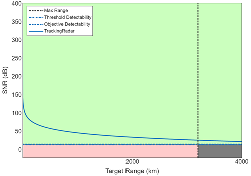
• SNR vs Range — View signal-to-noise ratio versus range for all designs

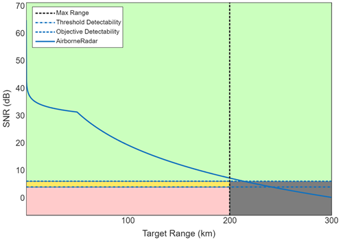
  To visualize the signal-to-noise ratio (SNR) as a function of range for your radar designs, click SNR vs Range on the toolstrip.

  Radar Designer displays the SNR in dB and shows the horizon range. The plot shows the maximum range requirements and a Stoplight Chart based on the detectability factor (required SNR) values.

  This plot shows the signal-to-noise ratio plot for one airborne radar with the default settings. For more information, see Radar Designer Configurations.

  

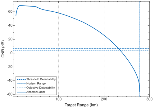
  To generate a script to recreate the signal-to-noise ratio plot for the currently selected radar, click Export on the toolstrip and select Export Detectability Analysis MATLAB Script.

• CNR vs Range — View clutter-to-noise ratio versus range for all designs

  To visualize the clutter-to-noise ratio (CNR) as a function of range for your radar designs, click CNR vs Range on the toolstrip.

  Radar Designer displays the CNR in dB and shows the horizon range.

  This plot shows the clutter-to-noise ratio plot for one airborne radar with an atmosphere over a land surface. For more information, see Radar Designer Configurations.

  

• Pd vs Range — Show probability of detection (P_d) versus range for all designs

  To visualize the probability of detection as a function of range for your radar designs, click Pd vs Range on the toolstrip.

  Radar Designer displays the probability of detection at the output of the receiver (effective P_d) as a function of the target range. The plot shows the maximum range requirements and a Stoplight Chart based on the desired P_d values.

  This plot shows the probability of detection versus range plot for one tracking radar with the default settings. For more information, see Radar Designer Configurations.

  

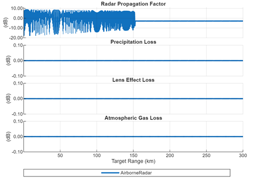
• Environmental Losses — View environmental losses for the currently selected radar

  To visualize the range-dependent loss components for your radar designs in their operation environments, click Environmental Losses on the toolstrip.

  Radar Designer displays four range-dependent loss components that correspond to different atmospheric and propagation effects:

  • Precipitation loss

  • Atmospheric gas loss

  • Lens-effect loss

  • Radar propagation factor

  This plot shows the environmental losses plot for one airport radar with the default settings using a high-latitude atmosphere model. For more information, see Radar Designer Configurations.

  

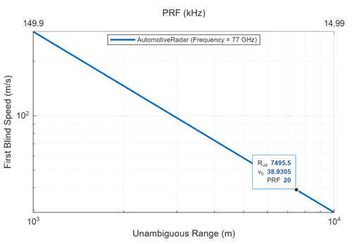
• Range/Doppler Coverage — Explore range/Doppler space for the currently selected radar

  To visualize the ambiguity-free range/Doppler coverage regions for your radar designs, click Range/Doppler Coverage on the toolstrip.

  Radar Designer displays a log-log plot of first blind speed as a function of unambiguous range (lower x-axis) and PRF (upper x-axis). Each solid line on the plot represents a radar design. Designs with different carrier frequencies appear as parallel lines.

  This plot shows the range/Doppler coverage plot for one automotive radar with the default settings. For more information, see Radar Designer Configurations.

  

Selected Radar — Display plots for selected radar

plot tab

View plots in the Selected Radar tab. By default, Radar Designer displays the Scenario Geometry plot.

Select additional plot types from the View Results gallery on the toolstrip.

Each selected plot will appear as a separate tab beneath Selected Radar. Toggle to Plots for Selected Radar using the arrow on the right hand side of the View Results gallery, if necessary.

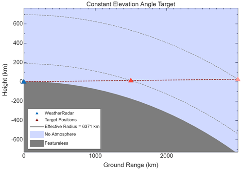
• Scenario Geometry — View scenario geometry for all designs

  To visualize the scenario geometry for your radar designs, click Scenario Geometry on the toolstrip.

  Radar Designer displays target height and position at various ranges (constant elevation angle). The radar antenna height, environment (effective Earth radius, free space), and radar antenna pattern demonstrating the applied tilt angle are also shown.

  This plot shows the scenario geometry plot for one weather radar with the default settings on a curved Earth. For more information, see Radar Designer Configurations.

  

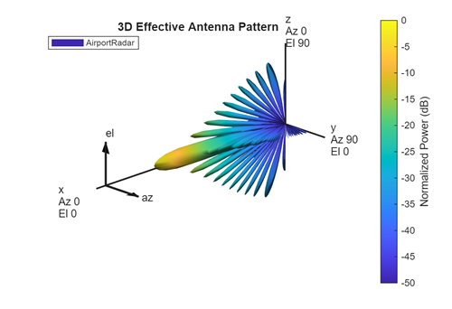
• Antenna Pattern — View 3D effective antenna pattern (since R2025a)

  To visualize the 3D effective antenna pattern for your radar designs, click Antenna Pattern on the toolstrip.

  Radar Designer displays the normalized antenna power radiation pattern in dB. The x-axis corresponds to a fixed azimuth angle of 0° and an elevation angle of 0°, the y-axis has an azimuth angle of 90° and an elevation angle of 0°, and the z-axis has an azimuth angle of 0° and an elevation of 90°.

  This plot shows the 3D antenna pattern plot for one airport radar with the default settings. For more information, see Radar Designer Configurations.

  

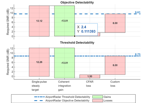
• Link Budget — Inspect gains and losses of the currently selected radar

  To visualize the gains and losses for your radar designs, click Link Budget on the toolstrip.

  Radar Designer models several components of the radar signal processing chain that affect the resulting Detectability Factor. The app displays a waterfall chart that shows the individual losses and gains that contribute to increasing the required signal energy. This chart is called the radar link budget.

  • The losses, represented in red, increase the required SNR threshold.

  • The gains, represented in green, decrease the required SNR threshold.

  Scan the plot left to right to see how the detectability factor changes as these components are added:

  • Steady-target single-pulse detectability

  • Integration gain

  • Fluctuation loss

  • Binary integration loss

  • CFAR loss

  • Eclipsing loss

  • MTI loss

  • Beam shape loss

  • Scan sector loss

  This plot shows the link budget plot for one airport radar with the default settings. For more information, see Radar Designer Configurations.

  

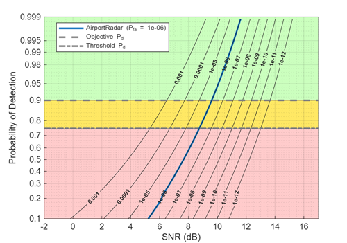
• Pd vs SNR — Show probability of detection (P_d) versus SNR for all designs.

  To visualize the probability of detection as a function of SNR for your radar designs, click Pd vs SNR on the toolstrip.

  Radar Designer displays the probability of detection at the output of the receiver (effective P_d) as a function of the received SNR. The plot shows the SNR requirements and a Stoplight Chart based on the desired P_d values.

  This plot shows the probability of detection versus SNR plot for one airport radar with the default settings. For more information, see Radar Designer Configurations.

  

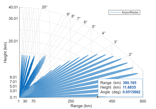
• Vertical Coverage — Plot Blake chart for the currently selected radar

  To visualize the range-height-angle relationships for your radar designs, click Vertical Coverage on the toolstrip.

  Radar Designer displays a vertical coverage diagram of the selected radar. Vertical coverage diagrams, also known as range-height-angle charts or Blake charts, show the relationship between the range to a target, the height of the target, and the initial elevation angle of the transmitted rays for the sensor.

  This plot shows the vertical coverage diagram for one airport radar with the curved earth model. For more information, see Radar Designer Configurations.

  

  To generate a script to recreate the vertical coverage plot for the currently selected radar, click Export on the toolstrip and select Export Vertical Coverage MATLAB Script.

Export Scripts

Export — Detectability analysis, vertical coverage, metrics report, and radarDataGenerator scripts

toolstrip button

Export to the MATLAB Workspace.

• Export Detectability Analysis MATLAB Script — Generate script to recreate SNR vs Range, Pd vs Range, Environmental Losses, and Link Budget plots

  To generate a script to recreate the signal-to-noise ratio, probability of detection, environmental losses, and link budget plots for the currently selected radar, click Export on the toolstrip and select Export Detectability Analysis MATLAB Script.

• Export Vertical Coverage MATLAB Script — Generate script to recreate vertical coverage plot

  To generate a script to recreate the vertical coverage plot for the currently selected radar, click Export on the toolstrip and select Export Vertical Coverage MATLAB Script.

• Generate Metrics Report — Generate formatted report of numeric metrics

  To generate a formatted report of numeric metrics for the currently selected radar, click Export on the toolstrip and select Generate Metrics Report.

• Export Radar Data Generator MATLAB Script — Generate script to simulate the selected radar detecting a target in a dynamic scenario (since R2024b)

  To generate a script that sets up a radarDataGenerator simulation within a radarScenario for the currently selected radar, click the Export button on the toolstrip and select Export Radar Data Generator MATLAB Script.

  The export script supports atmospheric refraction. Although Radar Designer uses the effective Earth radius model for atmospheric refraction calculations, radarDataGenerator also supports the CRPL exponential model. Therefore, you can select either Atmospheric Refraction Using Effective Earth Radius or Atmospheric Refraction Using CRPL Exponential Model in the Export Radar Data Generator MATLAB Script drop-down menu. To enable refraction, set Free Space to False and select an Atmosphere Model in the Radar Designer Environment tab. (since R2025a)

  Electronic and mechanical scanning radar configurations are also supported in the export script. (since R2025a)

Programmatic Use

radarDesigner

radarDesigner opens the Radar Designer app for designing radars, targets, and environment.

radarDesigner(sessionFileName)

radarDesigner(sessionFileName) opens the Radar Designer app and loads the specified radar file that was previously saved from the app.

More About

Radar Designer Configurations

Radar Designer includes radar configurations that enable you to switch between radar designs, duplicate radars, and delete radars.

This table shows the default parameter values for the built-in configurations.

Category	Property	Radar
		Airborne Radar	Airport Radar	Automotive Radar	Tracking Radar	Weather Radar
General	Icon
	Description	Long-range airborne surveillance radar	Terminal airport surveillance	Automotive radar for use in applications such as automatic cruise control	Ground-based, cued tracking radar system	Clear air weather radar
	Inspired By	Airborne scenario presented in [5]	ASR-9	Bosch LRR3, TI Radars	COBRA DANE	NEXRAD (VCP 32)
Main	Frequency	450 MHz	2.8 GHz	77 GHz	1.25 GHz	2.8 GHz
	Frequency band	UHF	S	W	L	S
	Bandwidth	4 MHz	1.5 MHz	300 MHz	20 MHz	0.5 MHz
	Peak power	200 kW	1.1 MW	30 mW	15 MW	500 kW
	Pulse width	200 μs	1 μs	50 μs	1 ms	1.5 μs
	PRF	300 Hz	1 kHz	20 kHz	1 kHz	320 Hz
Hardware	Noise temperature	1500 K (8 dB noise figure with reference temperature of 290K)	950 K	8000 K	800 K	450 K
Antenna and scanning	Antenna height	6096 m (20,000 ft)	10 m	1 m	75 m	20 m
	Antenna tilt	–1°	0.5°	0	10°	0.5°
	Polarization	Horizontal	Horizontal	Horizontal	Horizontal	Horizontal
	Gain	From beamwidth	From beamwidth	From beamwidth	From beamwidth	Manual
		Azimuth: 8°	Azimuth: 1.5°	Azimuth: 30°	Azimuth: 1°	45 dB
		Elevation: 90°	Elevation: 5°	Elevation: 10°	Elevation: 1°
	Scan mode	Electronic	Mechanical	N/A	N/A	Mechanical
		Azimuth ±30°	Full 360°			Volume scan: Azimuth: Full 360°. Elevation: 0.5° to 5°
	Scan time	0.05 s	5 s	N/A	N/A	10 minutes
Detection	Probability of false alarm	10–6	10–6	10–6	10–6	10–3
	Number of pulses in CPI	18	20	256	1	64
	Number of CPIs	1	1	1	1	1
Losses and other inputs	Custom loss	4 dB	8 dB	2 dB	2 dB	2 dB
	Other inputs	STC 'on' with default parameters	CFAR 'on' with default parameters	N/A	N/A	N/A
		CFAR 'on' with default parameters
		MTI 'on' with default parameters	MTI 'on' with default parameters
		Receive gain: 10 dB

Available Signal-to-Noise Ratio

The available signal-to-noise ratio at a range R, SNR_av(R), is the SNR at the input to the radar receiver after the transmitted radar signal has traveled through the medium, bounced off the target, and traveled back to the radar.

The available SNR is range-dependent and can be computed from the radar equation. The available SNR depends on radar operating frequency, transmitter power, pulse width, antenna gain, system noise temperature, and also on propagation losses and factors including atmospheric losses, eclipsing effects, and so on. The available SNR tells how much energy there is available for signal detection at the receiver.

Detectability Factor

The detectability factor or required SNR, D_x(P_d,P_fa), is the signal-to-noise ratio needed to detect a target with the desired probabilities of detection and false alarm.

The detectability factor is impacted by signal processing and scanning losses. Detection with the desired P_d and P_fa is possible when the available SNR is higher than the detectability factor. Plotting the available SNR and the detectability factor as a function of the range creates a clear image of the radar detection performance and shows the ranges in which detection is possible and those in which it is not.

Stoplight Chart

A radar system must meet a set of performance requirements that depend on the environment and scenarios in which the system is intended to operate. A number of such requirements can be fairly large and a design that satisfies all of them might be impractical. In this case a tradeoff analysis is applied. A subset of the requirements is satisfied at the expense of accepting lower values for the rest of the metrics. Such tradeoff analysis can be facilitated by specifying multiple requirement values for a single metric.

The requirement for each metric is specified as a pair of values:

• Objective — The desired level of the performance metric

• Threshold — The value of the metric below which the system's performance is considered unsatisfactory

The region between the Threshold and the Objective values is the trade-space. It defines a margin by which a metric can be below the Objective value while the system is still considered to have a satisfactory performance.

A stoplight chart color-codes the status of the performance metric for a radar system based on the specified requirements. The plot is divided into three zones:

• A Pass zone, colored green — At the ranges where the curve is in the Pass zone, the system performance satisfies the Objective value of the requirement.

• A Warn zone, colored yellow — At the ranges where the curve passes through the Warn zone, the system performance violates the Objective value of the specified requirement but still satisfies the Threshold value.

• A Fail zone, colored red — At the ranges where the curve passes through the Fail zone, the system performance violates the Threshold value of the specified requirement.

Tips

• Use Ctrl+Z to undo a modification. Use Ctrl+Y to redo an undone modification.

References

[1] Recommendation ITU-R P.835-6 (12/2017). "Reference Standard Atmospheres." Geneva: International Telecommunication Union, 2017.

[2] Barton, David K. Radar Equations for Modern Radar. Norwood, MA: Artech House, 2013.

[3] Gunn, K. L. S., and T. W. R. East. “The Microwave Properties of Precipitation Particles.” Quarterly Journal of the Royal Meteorological Society 80, no. 346 (October 1954): 522–45. https://doi.org/10.1002/qj.49708034603.

[4] O'Donnell, R. M. "Radar Systems Engineering." IEEE AES Society, IEEE New Hampshire Section, Radar Systems Course, January 2010.

[5] Ward, J. "Space-Time Adaptive Processing for Airborne Radar." TR-1015, MIT Lincoln Laboratory, December 1994. https://apps.dtic.mil/sti/tr/pdf/ADA293032.pdf

[6] Wasson, Charles S. System Engineering Analysis, Design, and Development: Concepts, Principles, and Practices. Second edition. Wiley Series in Systems Engineering and Management. Hoboken, New Jersey: John Wiley & Sons Inc, 2016.

Version History

Introduced in R2021a