Main Content

constantGammaClutter

Simulate constant gamma clutter

Since R2021a

Description

The constantGammaClutter object simulates clutter.

To compute the clutter return:

  1. Define and set up your clutter simulator. See Construction.

  2. Call step to simulate the clutter return for your system according to the properties of constantGammaClutter. The behavior of step is specific to each object in the toolbox.

The clutter simulation that constantGammaClutter provides is based on these assumptions:

  • The radar system is monostatic.

  • The propagation is in free space.

  • The terrain is homogeneous.

  • The clutter patch is stationary during the coherence time. Coherence time indicates how frequently the software changes the set of random numbers in the clutter simulation.

  • Because the signal is narrowband, the spatial response and Doppler shift can be approximated by phase shifts.

  • The radar system maintains a constant height during simulation.

  • The radar system maintains a constant speed during simulation.

Note

Starting in R2016b, instead of using the step method to perform the operation defined by the System object™, you can call the object with arguments, as if it were a function. For example, y = step(obj,x) and y = obj(x) perform equivalent operations.

Construction

H = constantGammaClutter creates a constant gamma clutter simulation System object, H. This object simulates the clutter return of a monostatic radar system using the constant gamma model.

H = constantGammaClutter(Name,Value) creates a constant gamma clutter simulation object, H, with additional options specified by one or more Name,Value pair arguments. Name is a property name, and Value is the corresponding value. Name must appear inside single quotes (''). You can specify several name-value pair arguments in any order as Name1,Value1,…,NameN,ValueN.

Properties

Sensor

Handle of sensor

Specify the sensor as an antenna element object or as an array object whose Element property value is an antenna element object. If the sensor is an array, it can contain subarrays.

Default: phased.ULA with default property values

Gamma

Terrain gamma value

Specify the γ value used in the constant γ clutter model, as a scalar in decibels. The γ value depends on both terrain type and the operating frequency.

Default: 0

EarthModel

Earth model

Specify the earth model used in clutter simulation as one of | 'Flat' | 'Curved' |. When you set this property to 'Flat', the earth is assumed to be a flat plane. When you set this property to 'Curved', the earth is assumed to be a sphere.

Default: 'Flat'

ClutterMinRange

Minimum range of clutter region (m)

Minimum range at which to computer clutter returns, specified as a positive scalar. The minimum range must be nonnegative. This value is ignored if it less than the value of PlatformHeight. Units are in meters.

Default: 0

ClutterMaxRange

Maximum range of clutter region (m)

Specify the maximum range at which to compute clutter returns. for the clutter simulation as a positive scalar. The maximum range must be greater than the value specified in the PlatformHeight property. Units are in meters.

Default: 5000

ClutterAzimuthCenter

Azimuth center of clutter region (deg)

The azimuth angle in the ground plane about which clutter patches are generated. Patches are generated symmetrically about this angle.

Default: 0

ClutterAzimuthSpan

Azimuth span of clutter region (deg)

Specify the coverage in azimuth (in degrees) of the clutter region as a positive scalar. The clutter simulation covers a region having the specified azimuth span, symmetric around ClutterAzimuthCenter. Typically, all clutter patches have their azimuth centers within the region, but the PatchAzimuthSpan value can cause some patches to extend beyond the region.

Default: 60

PatchAzimuthSpan

Azimuth span of clutter patches (deg)

Specify the azimuth span (in degrees) of each clutter patch as a positive scalar.

Default: 1

CoherenceTime

Clutter coherence time

Specify the coherence time in seconds for the clutter simulation as a positive scalar. After the coherence time elapses, the step method updates the random numbers it uses for the clutter simulation at the next pulse. A value of inf means the random numbers are never updated.

Default: inf

PropagationSpeed

Signal propagation speed

Specify the propagation speed of the signal, in meters per second, as a positive scalar.

Default: Speed of light

SampleRate

Sample rate

Specify the sample rate, in hertz, as a positive scalar. The default value corresponds to 1 MHz.

Default: 1e6

PRF

Pulse repetition frequency

Pulse repetition frequency, PRF, specified as a scalar or a row vector. Units are in Hz. The pulse repetition interval, PRI, is the inverse of the pulse repetition frequency, PRF. ThePRF must satisfy these restrictions:

  • The product of PRF and PulseWidth must be less than or equal to one. This condition expresses the requirement that the pulse width is less than one pulse repetition interval. For the phase-coded waveform, the pulse width is the product of the chip width and number of chips.

  • The ratio of sample rate to any element of PRF must be an integer. This condition expresses the requirement that the number of samples in one pulse repetition interval is an integer.

You can select the value of PRF using property settings alone or using property settings in conjunction with the prfidx input argument of the step method.

  • When PRFSelectionInputPort is false, you set the PRF using properties only. You can

    • implement a constant PRF by specifying PRF as a positive real-valued scalar.

    • implement a staggered PRF by specifying PRF as a row vector with positive real-valued entries. Then, each call to the step method uses successive elements of this vector for the PRF. If the last element of the vector is reached, the process continues cyclically with the first element of the vector.

  • When PRFSelectionInputPort is true, you can implement a selectable PRF by specifying PRF as a row vector with positive real-valued entries. But this time, when you execute the step method, select a PRF by passing an argument specifying an index into the PRF vector.

In all cases, the number of output samples is fixed when you set the OutputFormat property to 'Samples'. When you use a varying PRF and set the OutputFormat property to 'Pulses', the number of samples can vary.

Default: 10e3

PRFSelectionInputPort

Enable PRF selection input

Enable the PRF selection input, specified as true or false. When you set this property to false, the step method uses the values set in the PRF property. When you set this property to true, you pass an index argument into the step method to select a value from the PRF vector.

Default: false

OutputFormat

Output signal format

Specify the format of the output signal as one of | 'Pulses' | 'Samples' |. When you set the OutputFormat property to 'Pulses', the output of the step method is in the form of multiple pulses. In this case, the number of pulses is the value of the NumPulses property.

When you set the OutputFormat property to 'Samples', the output of the step method is in the form of multiple samples. In this case, the number of samples is the value of the NumSamples property. In staggered PRF applications, you might find the 'Samples' option more convenient because the step output always has the same matrix size.

Default: 'Pulses'

NumPulses

Number of pulses in output

Specify the number of pulses in the output of the step method as a positive integer. This property applies only when you set the OutputFormat property to 'Pulses'.

Default: 1

NumSamples

Number of samples in output

Specify the number of samples in the output of the step method as a positive integer. Typically, you use the number of samples in one pulse. This property applies only when you set the OutputFormat property to 'Samples'.

Default: 100

OperatingFrequency

System operating frequency

Specify the operating frequency of the system in hertz as a positive scalar. The default value corresponds to 300 MHz.

Default: 3e8

TransmitSignalInputPort

Add input to specify transmit signal

Set this property to true to add input to specify the transmit signal in the step syntax. Set this property to false omit the transmit signal in the step syntax. The false option is less computationally expensive; to use this option, you must also specify the TransmitERP property.

Default: false

WeightsInputPort

Enable weights input

Set this property to true to input weights.

Default: false

TransmitERP

Effective transmitted power

Specify the transmitted effective radiated power (ERP) of the radar system in watts as a positive scalar. This property applies only when you set the TransmitSignalInputPort property to false.

Default: 5000

PlatformHeight

Radar platform height from surface

Specify the radar platform height (in meters) measured upward from the surface as a nonnegative scalar.

Default: 300

PlatformSpeed

Radar platform speed

Specify the radar platform’s speed as a nonnegative scalar in meters per second.

Default: 300

PlatformDirection

Direction of radar platform motion

Specify the direction of radar platform motion as a 2-by-1 vector in the form [AzimuthAngle; ElevationAngle] in degrees. The default value of this property indicates that the platform moves perpendicular to the radar antenna array’s broadside.

Both azimuth and elevation angle are measured in the local coordinate system of the radar antenna or antenna array. Azimuth angle must be between –180 and 180 degrees. Elevation angle must be between –90 and 90 degrees.

Default: [90;0]

MountingAngles

Sensor mounting angles (deg)

Specify a 3-element vector that gives the intrinsic yaw, pitch, and roll of the sensor frame from the inertial frame. The 3 elements define the rotations around the z, y, and x axes respectively, in that order. The first rotation, rotates the body axes around the z-axis. Because these angles define intrinsic rotations, the second rotation is performed around the y-axis in its new position resulting from the previous rotation. The final rotation around the x-axis is performed around the x-axis as rotated by the first two rotations in the intrinsic system.

Default: [0 0 0]

SeedSource

Source of seed for random number generator

Specify how the object generates random numbers. Values of this property are:

'Auto'The default MATLAB® random number generator produces the random numbers. Use 'Auto' if you are using this object with Parallel Computing Toolbox™ software.
'Property'The object uses its own private random number generator to produce random numbers. The Seed property of this object specifies the seed of the random number generator. Use 'Property' if you want repeatable results and are not using this object with Parallel Computing Toolbox software.

Default: 'Auto'

Seed

Seed for random number generator

Specify the seed for the random number generator as a scalar integer between 0 and 232–1. This property applies when you set the SeedSource property to 'Property'.

Default: 0

Methods

Common to All System Objects
release

Allow System object property value changes

Examples

collapse all

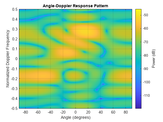
Simulate the clutter return from terrain with a gamma value of 0 dB. The effective transmitted power of the radar system is 5 kW.

Set up the characteristics of the radar system. This system uses a four-element uniform linear array (ULA). The sample rate is 1 MHz, and the PRF is 10 kHz. The propagation speed is the speed of light, and the operating frequency is 300 MHz. The radar platform is flying 1 km above the ground with a path parallel to the ground along the array axis. The platform speed is 2 km/s. The mainlobe has a depression angle of 30°.

Nele = 4;
c = physconst('Lightspeed');
fc = 300.0e6;
lambda = c/fc;
array = phased.ULA('NumElements',Nele,'ElementSpacing',lambda/2);
fs = 1.0e6;
prf = 10.0e3;
height = 1000.0;
direction = [90;0];
speed = 2.0e3;
depang = 30.0;
mountingAng = [depang,0,0];

Create the clutter simulation object. The configuration assumes the earth is flat. The maximum clutter range of interest is 5 km, and the maximum azimuth coverage is ±60°.

Rmax = 5000.0;
Azcov = 120.0;
tergamma = 0.0;
tpower = 5000.0;
clutter = constantGammaClutter('Sensor',array,...
    'PropagationSpeed',c,'OperatingFrequency',fc,'PRF',prf,...
    'SampleRate',fs,'Gamma',tergamma,'EarthModel','Flat',...
    'TransmitERP',tpower,'PlatformHeight',height,...
    'PlatformSpeed',speed,'PlatformDirection',direction,...
    'MountingAngles',mountingAng,'ClutterMaxRange',Rmax,...
    'ClutterAzimuthSpan',Azcov,'SeedSource','Property',...
    'Seed',40547);

Simulate the clutter return for 10 pulses.

Nsamp = fs/prf;
Npulse = 10;
sig = zeros(Nsamp,Nele,Npulse);
for m = 1:Npulse
    sig(:,:,m) = clutter();
end

Plot the angle-Doppler response of the clutter at the 20th range bin.

response = phased.AngleDopplerResponse('SensorArray',array,...
    'OperatingFrequency',fc,'PropagationSpeed',c,'PRF',prf);
plotResponse(response,shiftdim(sig(20,:,:)),'NormalizeDoppler',true)

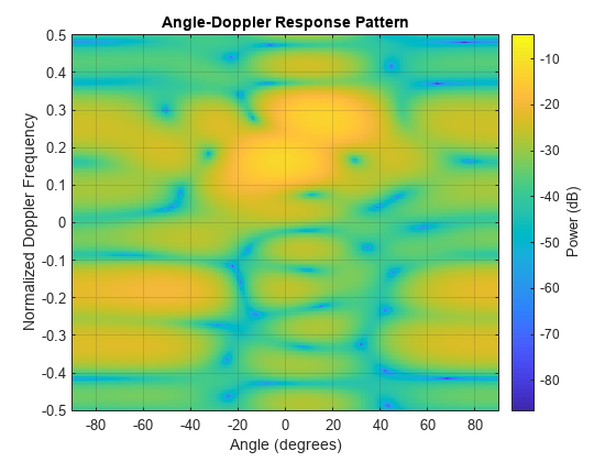
Simulate the clutter return from terrain with a gamma value of 0 dB. You input the transmit signal of the radar system when creating clutter. In this case, you do not use the TransmitERP property.

Set up the characteristics of the radar system. This system has a 4-element uniform linear array (ULA). The sample rate is 1 MHz, and the PRF is 10 kHz. The propagation speed is the speed of light, and the operating frequency is 300 MHz. The radar platform is flying 1 km above the ground with a path parallel to the ground along the array axis. The platform speed is 2 km/s. The mainlobe has a depression angle of 30°.

Nele = 4;
c = physconst('Lightspeed');
fc = 300.0e6;
lambda = c/fc;
ula = phased.ULA('NumElements',Nele,'ElementSpacing',lambda/2);
fs = 1.0e6;
prf = 10.0e3;
height = 1.0e3;
direction = [90;0];
speed = 2.0e3;
depang = 30;
mountingAng = [depang,0,0];

Create the clutter simulation object and configure it to accept an transmit signal as an input argument. The configuration assumes the earth is flat. The maximum clutter range of interest is 5 km, and the maximum azimuth coverage is ±60°.

Rmax = 5000.0;
Azcov = 120.0;
tergamma = 0.0;
clutter = constantGammaClutter('Sensor',ula,...
    'PropagationSpeed',c,'OperatingFrequency',fc,'PRF',prf,...
    'SampleRate',fs,'Gamma',tergamma,'EarthModel','Flat',...
    'TransmitSignalInputPort',true,'PlatformHeight',height,...
    'PlatformSpeed',speed,'PlatformDirection',direction,...
    'MountingAngles',mountingAng,'ClutterMaxRange',Rmax,...
    'ClutterAzimuthSpan',Azcov,'SeedSource','Property',...
    'Seed',40547);

Simulate the clutter return for 10 pulses. At each step, pass the transmit signal as an input argument. The software computes the effective transmitted power of the signal. The transmit signal is a rectangular waveform with a pulse width of 2 μs.

tpower = 5.0e3;
pw = 2.0e-6;
X = tpower*ones(floor(pw*fs),1);
Nsamp = fs/prf;
Npulse = 10;
sig = zeros(Nsamp,Nele,Npulse);
for m = 1:Npulse
    sig(:,:,m) = step(clutter,X);
end

Plot the angle-Doppler response of the clutter at the 20th range bin.

response = phased.AngleDopplerResponse('SensorArray',ula,...
    'OperatingFrequency',fc,'PropagationSpeed',c,'PRF',prf);
plotResponse(response,shiftdim(sig(20,:,:)),'NormalizeDoppler',true)

References

[1] Barton, David. “Land Clutter Models for Radar Design and Analysis,” Proceedings of the IEEE. Vol. 73, Number 2, February, 1985, pp. 198–204.

[2] Long, Maurice W. Radar Reflectivity of Land and Sea, 3rd Ed. Boston: Artech House, 2001.

[3] Nathanson, Fred E., J. Patrick Reilly, and Marvin N. Cohen. Radar Design Principles, 2nd Ed. Mendham, NJ: SciTech Publishing, 1999.

[4] Ward, J. “Space-Time Adaptive Processing for Airborne Radar Data Systems,” Technical Report 1015, MIT Lincoln Laboratory, December, 1994.

Extended Capabilities

Version History

Introduced in R2021a