phased.ULA
Uniform linear array
Description
phased.ULA creates a uniform linear array (ULA)
System object™ and computes its response.
To compute the response for each element in the array for specified directions:
Create the
phased.ULAobject and set its properties.Call the object with arguments, as if it were a function.
To learn more about how System objects work, see What Are System Objects?
Creation
Description
array = phased.ULAarray (ULA) System object. In this syntax, the object models a ULA formed with identical isotropic
phased array sensor elements. The origin of the local coordinate system is the phase
center of the array. The positive x-axis is the direction normal to the
array, and the elements of the array are located along the
y-axis.
array = phased.ULA(Name=Value)array with each specified property
Name set to the specified Value. You can
specify additional name-value pair arguments in any order as (Name1 =
Value1, … ,NameN =
ValueN).
array = phased.ULA(N,D,Name=Value)array object with the NumElements
property set to N, the ElementSpacing property
set to D, and other specified property Names set to the specified
Values. N and D are value-only arguments. When
specifying a value-only argument, specify all preceding value-only arguments. You can
specify name-value pair arguments in any order.
Properties
Usage
Syntax
Description
Input Arguments
Output Arguments
Object Functions
To use an object function, specify the
System object as the first input argument. For
example, to release system resources of a System object named obj, use
this syntax:
release(obj)
Examples
Compute the directivities of two different uniform linear arrays (ULA). One array consists of isotropic antenna elements and the second array consists of cosine antenna elements. In addition, compute the directivity when the first array is steered in a specified direction. For each case, calculate the directivities for a set of seven different azimuth directions all at zero degrees elevation. Set the frequency to 300 MHz.
Array of Isotropic Antenna Elements
First, create a 10-element ULA of isotropic antenna elements spaced 1/2-wavelength apart.
c = physconst("LightSpeed");
fc = 300e6;
lambda = c/fc;
ang = [-30,-20,-10,0,10,20,30; 0,0,0,0,0,0,0];
myAnt1 = phased.IsotropicAntennaElement;
myArray1 = phased.ULA(10,lambda/2,Element=myAnt1);
Compute the directivity.
d = directivity(myArray1,fc,ang,PropagationSpeed=c)
d = 7×1

   -6.9897
   -6.2294
   -6.5187
   10.0000
   -6.5187
   -6.2294
   -6.9897
Array of Cosine Antenna Elements
Next, create a 10-element ULA of cosine antenna elements spaced 1/2-wavelength apart.
myAnt2 = phased.CosineAntennaElement(CosinePower=[1.8,1.8]);
myArray2 = phased.ULA(10,lambda/2,Element=myAnt2);
Compute the directivity.
d = directivity(myArray2,fc,ang,PropagationSpeed=c)
d = 7×1

   -1.9838
    0.0529
    0.4968
   17.2548
    0.4968
    0.0529
   -1.9838
The directivity of the cosine ULA is greater than the directivity of the isotropic ULA because of the larger directivity of the cosine antenna element.
Steered Array of Isotropic Antenna Elements
Finally, steer the isotropic antenna array to 30 degrees in azimuth and compute the directivity.
w = steervec(getElementPosition(myArray1)/lambda,[30;0]);
d = directivity(myArray1,fc,ang,PropagationSpeed=c, ...
    Weights=w)
d = 7×1
-297.2705
-13.9783
-9.5713
-6.9897
-4.5787
-2.0537
10.0000
The directivity is greatest in the steered direction.
Construct three ULAs with elements along the x-, y-, and z-axes. Obtain the element normals.
First, choose the array axis along the x-axis.
sULA1 = phased.ULA(NumElements=5,ArrayAxis="x");
norm = getElementNormal(sULA1)
norm = 2×5
90 90 90 90 90
0 0 0 0 0
The element normal vectors point along the y-axis.
Next, choose the array axis along the y-axis.
sULA2 = phased.ULA(NumElements=5,ArrayAxis="y");
norm = getElementNormal(sULA2)
norm = 2×5
0 0 0 0 0
0 0 0 0 0
The element normal vectors point along the x-axis.
Finally, set the array axis along the z-axis. Obtain the normal vectors of the odd-numbered elements.
sULA3 = phased.ULA(NumElements=5,ArrayAxis="z");
norm = getElementNormal(sULA3,[1,3,5])
norm = 2×3
0 0 0
0 0 0
The element normal vectors also point along the x-axis.
Construct a ULA with 5 elements along the z-axis. Obtain the element positions.
array = phased.ULA(NumElements=5,ArrayAxis="z");
pos = getElementPosition(array)
pos = 3×5
0 0 0 0 0
0 0 0 0 0
-1.0000 -0.5000 0 0.5000 1.0000
Construct a default ULA and obtain the number of elements in that array.
 array = phased.ULA;
 N = getNumElements(array)
N =
2
Draw a 6-element ULA and use the ShowIndex parameter to show the indices of the first and third elements.
array = phased.ULA(6);
viewArray(array,ShowIndex=[1 3],ShowNormals=true, ...
    ShowLocalCoordinates=true,Orientation=[60;100;45], ...
    ShowAnnotation=true)

Construct a 5-element ULA with a Taylor window taper. Then, obtain the element taper values.
taper = taylorwin(5)';
array = phased.ULA(5,Taper=taper);
w = getTaper(array)
w = 5×1

    0.5181
    1.2029
    1.5581
    1.2029
    0.5181
Show that an array of phased.ShortDipoleAntennaElement antenna elements supports polarization.
antenna = phased.ShortDipoleAntennaElement(...
    FrequencyRange=[1e9 10e9]);
array = phased.ULA(NumElements=3,Element=antenna);
isPolarizationCapable(array)
ans = logical
1
The returned value of 1 shows that this array supports polarization.
Create a 4-element undersampled ULA and find the response of each element at boresight. Plot the array pattern at 1 GHz for azimuth angles between -180 and 180 degrees. The default element spacing is 0.5 meters.
array = phased.ULA(NumElements=4); fc = 1e9; ang = [0;0]; resp = array(fc,ang)
resp = 4×1
1
1
1
1
c = physconst("LightSpeed"); pattern(array,fc,-180:180,0,PropagationSpeed=c, ... CoordinateSystem="rectangular", ... Type="powerdb",Normalize=true)

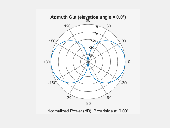
Construct a 10-element uniform linear array of omnidirectional microphones spaced 3 cm apart. Then, plot the array pattern at 100 Hz.
mic = phased.OmnidirectionalMicrophoneElement(... FrequencyRange=[20 20e3]); Nele = 10; array = phased.ULA(NumElements=Nele, ... ElementSpacing=3e-2, ... Element=mic); fc = 100; ang = [0; 0]; resp = array(fc,ang); c = 340; pattern(array,fc,[-180:180],0,PropagationSpeed=c, ... CoordinateSystem="polar", ... Type="powerdb", ... Normalize=true);

Build a tapered uniform line array of 5 short-dipole sensor elements. Because short dipoles support polarization, the array should as well. Verify that it supports polarization by looking at the output of the isPolarizationCapable method.
antenna = phased.ShortDipoleAntennaElement(... 'FrequencyRange',[100e6 1e9],'AxisDirection','Z'); array = phased.ULA('NumElements',5,'Element',antenna,... 'Taper',[.5,.7,1,.7,.5]); isPolarizationCapable(array)
ans = logical
   1
Then, draw the array using the viewArray method.
viewArray(array,'ShowTaper',true,'ShowIndex','All')

Compute the horizontal and vertical responses.
fc = 150e6;
ang = [10];
resp = array(fc,ang);
Display the horizontal polarization response.
resp.H
ans = 5×1

     0
     0
     0
     0
     0
Display the vertical polarization response.
resp.V
ans = 5×1

   -0.6124
   -0.8573
   -1.2247
   -0.8573
   -0.6124
Plot an azimuth cut of the vertical polarization response.
c = physconst('LightSpeed');
pattern(array,fc,[-180:180],0,...
    'PropagationSpeed',c,...
    'CoordinateSystem','polar',...
    'Polarization','V',...
    'Type','powerdb',...
    'Normalize',true)
Create an 9-element ULA of short dipole antenna elements spaced 1.5 meters apart. Display the azimuth and elevation directivities. The operating frequency is 500 MHz. Plot the directivities in polar coordinates.
Evaluate the fields at 45° azimuth and 0° elevation.
element = phased.ShortDipoleAntennaElement(...
    FrequencyRange=[50e6,1000e6], ...
    AxisDirection="Z");
array = phased.ULA(NumElements=9,ElementSpacing=1.5,Element=element);
fc = 500e6;
ang = [45;0];
resp = array(fc,ang);
disp(resp.V)
   -1.2247
   -1.2247
   -1.2247
   -1.2247
   -1.2247
   -1.2247
   -1.2247
   -1.2247
   -1.2247
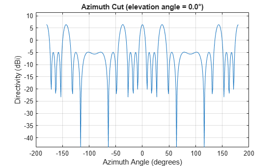
Display the azimuth directivity pattern at 500 MHz for azimuth angles between -180° and 180°.
c = physconst("LightSpeed");
pattern(array,fc,[-180:180],0, ...
    Type="directivity", ...
    PropagationSpeed=c)
Display the elevation directivity pattern at 500 MHz for elevation angles between -90° and 90°.
pattern(array,fc,[0],[-90:90], ...
    Type="directivity", ...
    PropagationSpeed=c)
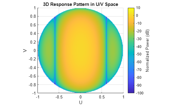
Create a 10-element ULA antenna array consisting of cosine antenna elements spaced 10 cm apart. Display the 3-D power pattern in UV space. The operating frequency is 500 MHz.
sCos = phased.CosineAntennaElement(FrequencyRange=[100e6 1e9], ...
    CosinePower=[2.5,2.5]);
sULA = phased.ULA(NumElements=10, ...
    ElementSpacing=.1, ...
    Element=sCos);
c = physconst("LightSpeed");
fc = 500e6;
pattern(sULA,fc,[-1:.01:1],[-1:.01:1], ...
    CoordinateSystem="uv", ...
    Type="powerdb", ...
    PropagationSpeed=c)
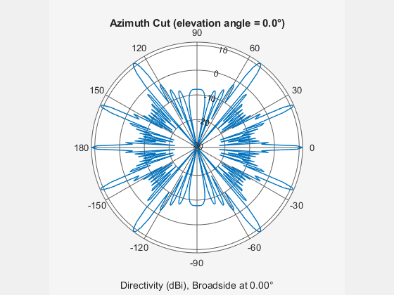
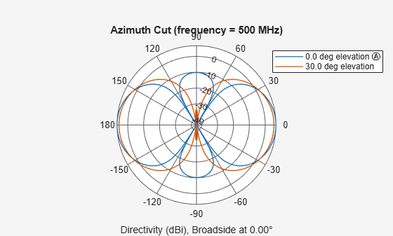
Create a 7-element ULA of short-dipole antenna elements spaced 10 cm apart. Plot an azimuth cut of directivity at 0° and 10° elevation. Assume the operating frequency is 500 MHz.
fc = 500e6;
sCDant = phased.ShortDipoleAntennaElement(FrequencyRange=[100,900]*1e6);
sULA = phased.ULA(NumElements=7,ElementSpacing=0.1,Element=sCDant);
patternAzimuth(sULA,fc,[0 30])
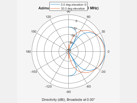
You can plot a smaller range of azimuth angles by setting the Azimuth property.
patternAzimuth(sULA,fc,[0 30],Azimuth=[-90:90])
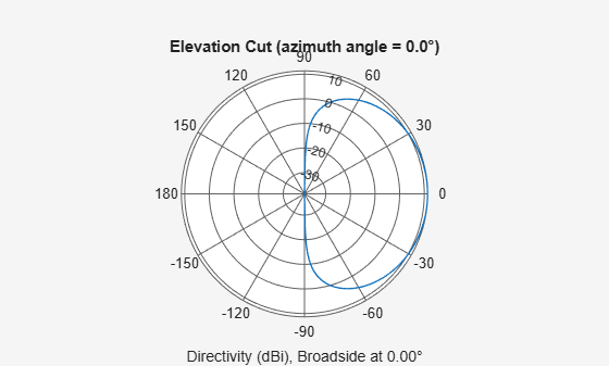
Create a 6-element ULA of short-dipole antenna elements with element spacing of 10 cm. Plot an elevation cut of directivity at 0° and 90° azimuth. Assume the operating frequency is 500 MHz.
fc = 500e6;
c = physconst("LightSpeed");
elem = phased.ShortDipoleAntennaElement(FrequencyRange=[100,900]*1e6);
array= phased.ULA(NumElements=6,ElementSpacing=0.1,Element=elem);
patternElevation(array,fc,[0 90],PropagationSpeed=c)
legend("Location","southwest")

You can plot a smaller range of elevation angles by setting the Elevation property to [0:90] degrees but now with cuts at 0° and 45° azimuth.
patternElevation(array,fc,[0 45],Elevation=[0:90],PropagationSpeed=c)
legend("Location","southwest")

Plot the beamwidth of a sonar array operating at a frequency of 2 kHz when the propagation speed of sound in water is 1500 m/s.
The sonar array consists of a 20-element uniform linear array (ULA). Consider the element of the ULA to be a backbaffled phased.IsotropicProjector with a VoltageResponse of 100 Volts and with a FrequencyRange from 10 Hz to 300 kHz. Create a phased.ULA object to model the uniform linear array.
 projector = phased.IsotropicProjector(BackBaffled=true, ...
        VoltageResponse=100,FrequencyRange=[10 300000])
projector =
phased.IsotropicProjector with properties:
VoltageResponse: 100
FrequencyRange: [10 300000]
BackBaffled: true
myArray = phased.ULA(Element=projector,NumElements=20, ...
    ElementSpacing=1500/200e3/2)
myArray =
phased.ULA with properties:
Element: [1×1 phased.IsotropicProjector]
NumElements: 20
ElementSpacing: 0.0037
ArrayAxis: 'y'
Taper: 1
Using the beamwidth function, calculate and plot the 6 dB beamwidth of the sonar array.
beamwidth(myArray,200e3,dBDown=6,PropagationSpeed=1500)

ans =
6.9200
Calculate the half-power beamwidth and angles of a 20-element uniform linear array (ULA) of cosine antenna elements.
Create a phased.CosineAntennaElement object with the CosinePower exponents set to 1.5.
myAnt = phased.CosineAntennaElement
myAnt =
  phased.CosineAntennaElement with properties:

    FrequencyRange: [0 1.0000e+20]
       CosinePower: [1.5000 1.5000]
Create a phased.ULA object to model a 20-element ULA of cosine antenna elements. These elements are spaced at 0.5 meters on the azimuth plane.
array = phased.ULA(Element=myAnt,NumElements=20)
array =
  phased.ULA with properties:

           Element: [1×1 phased.CosineAntennaElement]
       NumElements: 20
    ElementSpacing: 0.5000
         ArrayAxis: 'y'
             Taper: 1
Compute the beamwidth and angles of the array when it is operating at 3e8 Hz. Specify the beamwidth to be computed along the elevation plane.
[BW,Ang] = beamwidth(array,3e8,Cut="Elevation")BW = 74.8200
Ang = 1×2

  -37.4100   37.4100
Create a 4-element ULA of isotropic antenna elements and find the response of each element at boresight. Plot the array response at 1 GHz for azimuth angles between -180° and 180°.
ha = phased.ULA(NumElements=4);
fc = 1e9;
ang = [0;0];
resp = ha(fc,ang);
c = physconst("LightSpeed");
pattern(ha,fc,[-180:180],0, ...
    PropagationSpeed=c, ...
    CoordinateSystem="rectangular")
Find the response of a ULA array of 10 omnidirectional microphones spaced 1.5 meters apart. Set the frequency response of the microphone to the range 20 Hz to 20 kHz and choose the signal frequency to be 100 Hz. Using the step method, determine the response of each element at boresight: 0 degrees azimuth and 0 degrees elevation.
mic = phased.OmnidirectionalMicrophoneElement( ...
    FrequencyRange=[20 20e3]);
Nelem = 10;
array = phased.ULA(NumElements=Nelem, ...
    ElementSpacing=1.5,Element=mic);
fc = 100;
ang = [0;0];
resp = array(fc,ang)
resp = 10×1

     1
     1
     1
     1
     1
     1
     1
     1
     1
     1
Plot the array directivity. Assume the speed of sound in air to be 340 m/s.
c = 340;
pattern(array,fc,[-180:180],0,PropagationSpeed=c,CoordinateSystem="polar")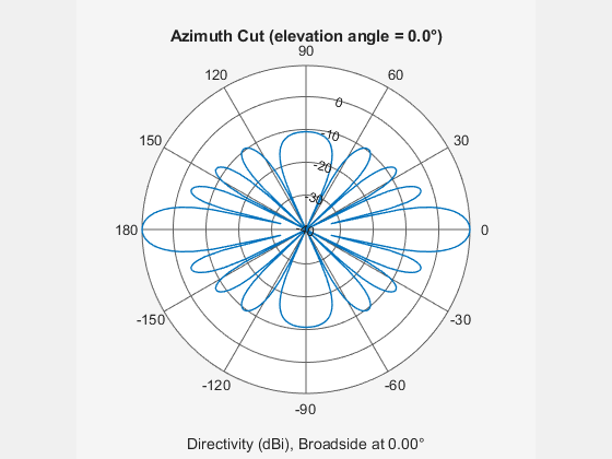
Simulate two received plane-wave random signals at a 4-element ULA. The signals arrive from 10° and 30° azimuth. Both signals have an elevation angle of 0°. Assume the propagation speed is the speed of light and the carrier frequency of the signal is 100 MHz.
array = phased.ULA(4);
y = collectPlaneWave(array,randn(4,2),[10 30],100e6,physconst("LightSpeed"))
y = 4×4 complex
0.7430 - 0.3705i 0.8433 - 0.1314i 0.8433 + 0.1314i 0.7430 + 0.3705i
0.8418 + 0.4308i 0.5632 + 0.1721i 0.5632 - 0.1721i 0.8418 - 0.4308i
-2.4817 + 0.9157i -2.6683 + 0.3175i -2.6683 - 0.3175i -2.4817 - 0.9157i
1.0724 - 0.4748i 1.1895 - 0.1671i 1.1895 + 0.1671i 1.0724 + 0.4748i
Plot the grating lobe diagram for a 4-element uniform linear array having element spacing less than one-half wavelength. Grating lobes are plotted in u-v coordinates.
Assume the operating frequency of the array is 3 GHz and the spacing between elements is 0.45 of the wavelength. All elements are isotropic antenna elements. Steer the array in the direction 45° in azimuth and 0° in elevation.
c = physconst("LightSpeed");
f = 3e9;
lambda = c/f;
sIso = phased.IsotropicAntennaElement;
sULA = phased.ULA(Element=sIso,NumElements=4, ...
    ElementSpacing=0.45*lambda);
plotGratingLobeDiagram(sULA,f,[45;0],c);
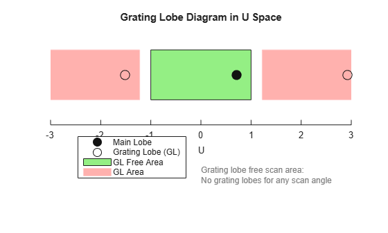
The main lobe of the array is indicated by a filled black circle. The grating lobes in the visible and nonvisible regions are indicated by empty black circles. The visible region is defined by the direction cosine limits between [-1,1] and is marked by the two vertical black lines. Because the array spacing is less than one-half wavelength, there are no grating lobes in the visible region of space. There are an infinite number of grating lobes in the nonvisible regions, but only those in the range [-3,3] are shown.
The grating-lobe free region, shown in green, is the range of directions of the main lobe for which there are no grating lobes in the visible region. In this case, it coincides with the visible region.
The white area of the diagram indicates a region where no grating lobes are possible.
Plot the grating lobe diagram for a 4-element uniform linear array having element spacing greater than one-half wavelength. Grating lobes are plotted in u-v coordinates.
Assume the operating frequency of the array is 3 GHz and the spacing between elements is 0.65 of a wavelength. All elements are isotropic antenna elements. Steer the array in the direction 45° in azimuth and 0° in elevation.
c = physconst("LightSpeed");
f = 3e9;
lambda = c/f;
sIso = phased.IsotropicAntennaElement;
sULA = phased.ULA(Element=sIso,NumElements=4,ElementSpacing=0.65*lambda);
plotGratingLobeDiagram(sULA,f,[45;0],c);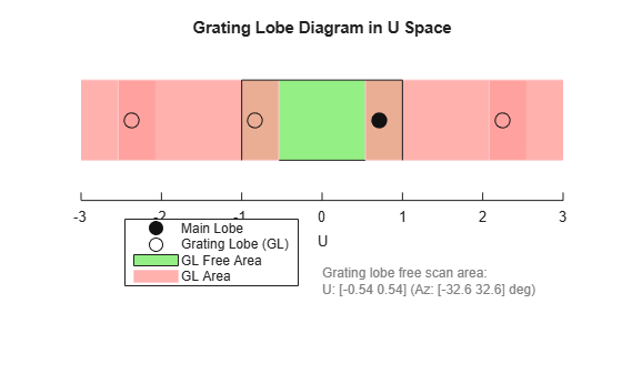
The main lobe of the array is indicated by a filled black circle. The grating lobes in the visible and nonvisible regions are indicated by empty black circles. The visible region, marked by the two black vertical lines, corresponds to arrival angles between -90 and 90 degrees. The visible region is defined by the direction cosine limits . Because the array spacing is greater than one-half wavelength, there is now a grating lobe in the visible region of space. There are an infinite number of grating lobes in the nonvisible regions, but only those for which are shown.
The grating-lobe free region, shown in green, is the range of directions of the main lobe for which there are no grating lobes in the visible region. In this case, it lies inside the visible region.
Plot the grating lobe diagram for a 4-element uniform linear array having element spacing greater than one-half wavelength. Apply a phase-shifter frequency that differs from the signal frequency. Grating lobes are plotted in u-v coordinates.
Assume the signal frequency is 3 GHz and the spacing between elements is 0.65 . All elements are isotropic antenna elements. The phase-shifter frequency is set to 3.5 GHz. Steer the array in the direction azimuth, elevation.
c = physconst("LightSpeed");
f = 3e9;
f0 = 3.5e9;
lambda = c/f;
sIso = phased.IsotropicAntennaElement;
sULA = phased.ULA(Element=sIso,NumElements=4, ...
    ElementSpacing=0.65*lambda);
plotGratingLobeDiagram(sULA,f,[45;0],c,f0);
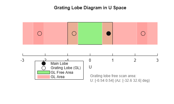
As a result of adding the shifted frequency, the mainlobe shifts right towards larger values. The beam no longer points toward the actual source arrival angle.
The mainlobe of the array is indicated by a filled black circle. The grating lobes in the visible and nonvisible regions are indicated by empty black circles. The visible region, marked by the two black vertical lines, corresponds to arrival angles between and . The visible region is defined by the direction cosine limits . Because the array spacing is greater than one-half wavelength, there is now a grating lobe in the visible region of space. There are an infinite number of grating lobes in the nonvisible regions, but only those for which are shown.
The grating-lobe free region, shown in green, is the range of directions of the main lobe for which there are no grating lobes in the visible region. In this case, it lies inside the visible region.
References
[1] Brookner, E., ed. Radar Technology. Lexington, MA: LexBook, 1996.
[2] Van Trees, H. Optimum Array Processing. New York: Wiley-Interscience, 2002.
Extended Capabilities
Version History
Introduced in R2011aSee Also
phased.ReplicatedSubarray | phased.PartitionedArray | phased.ConformalArray | phased.CosineAntennaElement | phased.CustomAntennaElement | phased.CrossedDipoleAntennaElement | phased.IsotropicAntennaElement | phased.ShortDipoleAntennaElement | phased.URA | phased.UCA | phased.HeterogeneousULA | phased.HeterogeneousURA | sidelobelevel