Main Content

phased.MUSICEstimator

Estimate direction of arrival using narrowband MUSIC algorithm for ULA

Description

The phased.MUSICEstimator System object™ implements the narrowband multiple signal classification (MUSIC) algorithm for uniform linear arrays (ULA). MUSIC is a high-resolution direction-finding algorithm capable of resolving closely-spaced signal sources. The algorithm uses eigenspace decomposition of the sensor spatial covariance matrix.

To estimate directions of arrival (DOA):

  1. Create the phased.MUSICEstimator object and set its properties.

  2. Call the object with arguments, as if it were a function.

To learn more about how System objects work, see What Are System Objects?

Creation

Description

musicEstimator = phased.MUSICEstimator creates a MUSIC DOA estimator System object, musicEstimator.

musicEstimator = phased.MUSICEstimator(Name=Value) sets properties using one or more optional name-value arguments. For example, OperatingFrequency=4e8 sets the operating frequency to 4e8.

example

Properties

expand all

Unless otherwise indicated, properties are nontunable, which means you cannot change their values after calling the object. Objects lock when you call them, and the release function unlocks them.

If a property is tunable, you can change its value at any time.

For more information on changing property values, see System Design in MATLAB Using System Objects.

ULA sensor array, specified as a phased.ULA object.

Signal propagation speed, specified as a positive scalar. The units are in meters per second.

Data Types: single | double

System operating frequency, specified as a positive scalar. The units are in hertz.

Data Types: single | double

Forward-backward averaging option, specified as true (logical 1) or false (logical 0). When you set this property to true, the object uses forward-backward averaging to estimate the covariance matrix for sensor arrays with conjugate symmetric array manifold.

Data Types: logical

Scan angles, specified as a vector of broadside angles in the range [−90, 90]. The units are in degrees. Broadside angles are between the search direction and the ULA array axis. You must specify the angles in ascending order.

Data Types: single | double

DOA output activation, specified as true (logical 1) or false (logical 0). To obtain the DOA of the signal, set this property to true and use the corresponding output argument when invoking the object ( as if it were a function). If you do not want to obtain the DOA, set this property to false. When you invoke the object, it returns the DOAs in the second output argument.

Data Types: logical

Source of the number of signals, specified as one of these options.

  • "Auto" — The object estimates the number of arriving signals using the method specified in the NumSignalsMethod property.

  • "Property" — You can specify the number of arriving signals using the NumSignals property.

Method to estimate the number of signals, specified as "AIC" or "MDL". The "AIC" uses the Akaike Information Criterion and the "MDL" uses Minimum Description Length criterion.

Dependencies

This property applies when you set the NumSignalsSource property to "Auto".

Number of arriving signals for the DOA estimation, specified as a positive integer.

Dependencies

This property applies when you set the NumSignalsSource property to "Property".

Data Types: single | double

Option to enable spatial smoothing, specified as a nonnegative integer. Use spatial smoothing to compute the arrival directions of coherent signals. A value of zero indicates no spatial smoothing. A positive value represents the number of subarrays used to compute the smoothed (averaged) source covariance matrix. Each increment in this value lets you handle one additional coherent source, but reduces the effective number of array elements by one. The length of the smoothing aperture, L, depends on the array length, M, and the averaging number, K, by L = M – K + 1. The maximum value of K is M – 2.

Example: 5

Data Types: double

Usage

Description

spectrum = musicEstimator(X) returns the MUSIC spectrum for a signal, X.

[spectrum,doa] = musicEstimator(X) additionally returns the signal broadside directions of arrival, doa. To use this syntax, set the DOAOutputPort property to true.

Note

The object performs an initialization the first time the object is executed. This initialization locks nontunable properties and input specifications, such as dimensions, complexity, and data type of the input data. If you change a nontunable property or an input specification, the System object issues an error. To change nontunable properties or inputs, you must first call the release method to unlock the object.

Input Arguments

expand all

Received signal, specified as an M-by-N complex-valued matrix. The quantity M is the number of sample values (snapshots) contained in the signal, and N is the number of sensor elements in the array.

The size of the first dimension of the input matrix can vary to simulate a changing signal length. A size change can occur, for example, in the case of a pulse waveform with variable pulse repetition frequency.

Example: [[0;1;2;3;4;3;2;1;0],[1;2;3;4;3;2;1;0;0]]

Data Types: double
Complex Number Support: Yes

Output Arguments

expand all

MUSIC spatial spectrum, returned as a nonnegative, real-valued K-element column vector representing the magnitude of the estimated MUSIC spatial spectrum. Each entry corresponds to an angle specified by the ScanAngles property.

Directions of arrival of the signals, returned as a real-valued L-element row vector. The direction of arrival angle is the angle between the source direction and the array axis or broadside angle. The units are in degrees. L is the number of signals specified by the NumSignals property or computed using the method specified by the NumSignalsMethod property.

Dependencies

To enable this output argument, set the DOAOutputPort property to true.

Object Functions

To use an object function, specify the System object as the first input argument. For example, to release system resources of a System object named obj, use this syntax:

release(obj)

expand all

plotSpectrumPlot MUSIC spectrum
stepRun System object algorithm
releaseRelease resources and allow changes to System object property values and input characteristics
resetReset internal states of System object

Examples

collapse all

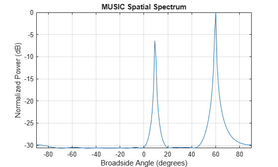
Estimate the DOAs of two signals received by a standard 10-element ULA having an element spacing of 1 meter. Then plot the MUSIC spectrum.

Create a ULA array object. The antenna operating frequency is 150 MHz.

fc = 150.0e6;
array = phased.ULA(NumElements=10,ElementSpacing=1.0);

Create the arriving signals at the ULA. The true direction of arrival of the first signal is 10° in azimuth and 20° in elevation. The direction of the second signal is 60° in azimuth and -5° in elevation.

fs = 8000.0;
t = (0:1/fs:1).';
sig1 = cos(2*pi*t*300.0);
sig2 = cos(2*pi*t*400.0);
sig = collectPlaneWave(array,[sig1 sig2],[10 20; 60 -5]',fc);
noise = 0.1*(randn(size(sig)) + 1i*randn(size(sig)));

Estimate the DOAs.

estimator = phased.MUSICEstimator(SensorArray=array,...
    OperatingFrequency=fc,...
    DOAOutputPort=true,NumSignalsSource="Property",...
    NumSignals=2);
[y,doas] = estimator(sig + noise);
doas = broadside2az(sort(doas),[20 -5])
doas = 1×2

    9.5829   60.3813

Plot the MUSIC spectrum.

plotSpectrum(estimator,"NormalizeResponse",true)

Figure contains an axes object. The axes object with title MUSIC Spatial Spectrum, xlabel Broadside Angle (degrees), ylabel Normalized Power (dB) contains an object of type line. This object represents 1 GHz.

First, estimate the DOAs of two signals received by a standard 10-element ULA having an element spacing of one-half wavelength.Then, plot the spatial spectrum.

The antenna operating frequency is 150 MHz. The arrival directions of the two signals are separated by 2°. The direction of the first signal is 30° azimuth and 0° elevation. The direction of the second signal is 32° azimuth and 0° elevation. Estimate the number of signals using the Minimum Description Length (MDL) criterion.

Create the signals arriving at the ULA.

fs = 8000;
t = (0:1/fs:1).';
f1 = 300.0;
f2 = 600.0;
sig1 = cos(2*pi*t*f1);
sig2 = cos(2*pi*t*f2);
fc = 150.0e6;
c = physconst('LightSpeed');
lam = c/fc;
array = phased.ULA('NumElements',10,'ElementSpacing',0.5*lam);
sig = collectPlaneWave(array,[sig1 sig2],[30 0; 32 0]',fc);
noise = 0.1*(randn(size(sig)) + 1i*randn(size(sig)));

Estimate the DOAs.

estimator = phased.MUSICEstimator('SensorArray',array,...
    'OperatingFrequency',fc,'DOAOutputPort',true,...
    'NumSignalsSource','Auto','NumSignalsMethod','MDL');
[y,doas] = estimator(sig + noise);
doas = broadside2az(sort(doas),[0 0])
doas = 1×2

   30.0000   32.0000

Plot the MUSIC spectrum.

plotSpectrum(estimator,'NormalizeResponse',true)
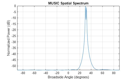
Figure contains an axes object. The axes object with title MUSIC Spatial Spectrum, xlabel Broadside Angle (degrees), ylabel Normalized Power (dB) contains an object of type line. This object represents 1 GHz.

Algorithms

expand all

References

[1] Van Trees, H. L. Optimum Array Processing. New York: Wiley-Interscience, 2002.

Extended Capabilities

expand all

Version History

Introduced in R2016b