Static and Animated Plots with Visualize PDE Results Live Editor Task

This example shows how to create an animated plot by using the Visualize PDE Results Live Editor task. The example solves a thermal analysis problem on a heat sink geometry, plots the temperature distribution at four time steps, and generates code for the visualization created by the Live Editor task. You can copy the generated code, modify and adapt the code for your problems, and use the code both in a live script and outside of a live script. The example also shows how to export an animation to a movie or an animated GIF file.

Create Geometry

Create the geometry representing a heat sink. Define the geometry description matrix for the rectangle and 11 circles.

gd = zeros(10,11);
gd(:,1) = [3 4 0 0.01 0.01 0 0 0 0.008 0.008];
k = 2;
for i = 0.002:0.002:0.008
   for j = 0.002:0.002:0.006
       gd(:,k)=[1 i j 0.0005 0 0 0 0 0 0];
       k = k + 1;
   end
end

Define the set formula and the name-space matrix.

sf='R1+C1+C2+C3+C4+C5+C6+C7+C8+C9+C10+C11+C12';
ns = ["R1" "C1" "C2" "C3" "C4" "C5" "C6" ...
      "C7" "C8" "C9" "C10" "C11" "C12"];

Create a 2-D geometry from the decomposed geometry matrix.

g = fegeometry(decsg(gd,sf,ns));

Plot the geometry with face labels.

pdegplot(g,FaceLabels="on")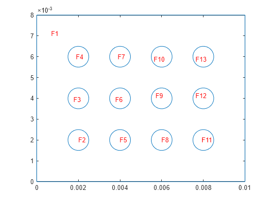

Extrude the 2-D geometry along the z-axis by 0.0005 units.

g = extrude(g,0.0005);

Plot the extruded geometry so that you can see the face labels on top.

figure
pdegplot(g,FaceLabels="on")
view([0 90])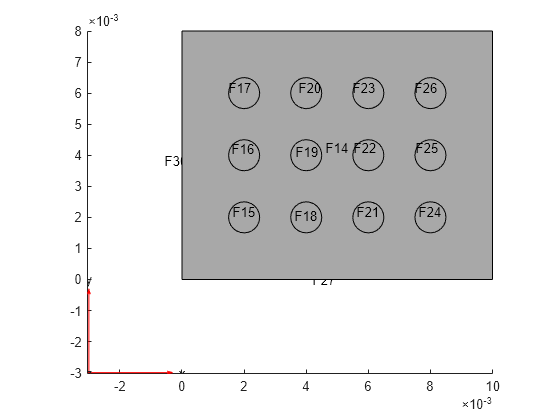

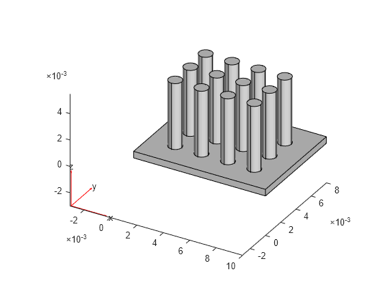
Extrude the circular faces (faces with IDs from 15 to 26) along the z-axis by 0.005 more units. These faces form the fins of the heat sink.

g = extrude(g,15:26,0.005);

Plot the geometry.

figure
pdegplot(g)

Perform Thermal Analysis

Create an femodel object for transient thermal analysis and include the geometry.

model = femodel(AnalysisType="thermalTransient", ...
    Geometry = g);

Assuming that the heat sink is made of copper, specify the thermal conductivity, mass density, and specific heat.

model.MaterialProperties = ...
    materialProperties(ThermalConductivity=400, ...
    MassDensity=8960, ...
    SpecificHeat=386);

Specify the Stefan-Boltzmann constant.

model.StefanBoltzmann = 5.670367e-8;

Apply the temperature boundary condition on the bottom surface of the heat sink, which consists of 13 faces.

model.FaceBC(1:13) = faceBC(Temperature=1000);

Specify the convection and radiation parameters on all other surfaces of the heat sink.

model.FaceLoad(14:g.NumFaces) = ...
    faceLoad(ConvectionCoefficient=5, ...
    AmbientTemperature=300, ...
    Emissivity=0.8);

Set the initial temperature of all the surfaces to the ambient temperature.

model.CellIC = cellIC(Temperature=300);

Generate a mesh.

model = generateMesh(model);

Solve the transient thermal problem for times between 0 and 0.0075 s with a time step of 0.0025 s.

results = solve(model,0:0.0025:0.0075);

Plot and Animate Resulting Temperatures

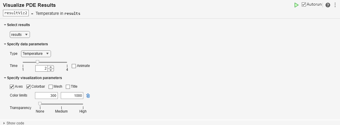
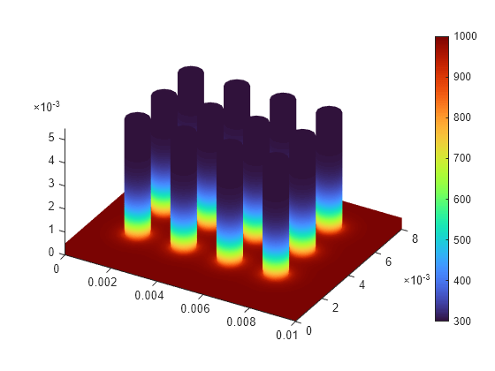
Plot the temperature distribution by using the Visualize PDE Results Live Editor task. First, because you specified a small number of time steps when calculating the solution, set the minimum number of frames needed to show playback buttons to 2. If an animation contains fewer frames than the specified minimum number, playback controls do not appear for that animation.

s = settings;
s.matlab.editor.MinimumFramesForAnimation.TemporaryValue = 2;

Create a new live script by clicking the New Live Script button in the File section on the Home tab.

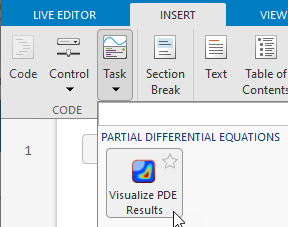
On the Live Editor tab, select Task > Visualize PDE Results. The software inserts the task into your script.

To plot the temperature distribution for each time step, complete these steps:

1. In the Select results section of the task, select results from the list.

2. In the Specify data parameters section of the task, set Type to Temperature, and select a time step from 1, 2, 3, and 4. These time steps correspond to the four time values that you used to solve the problem. For example, select step 2.

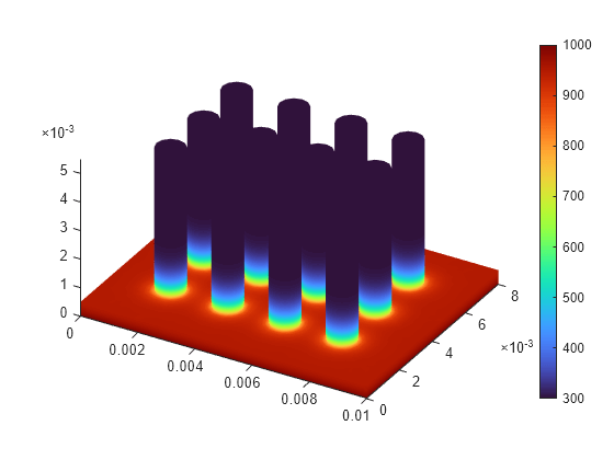
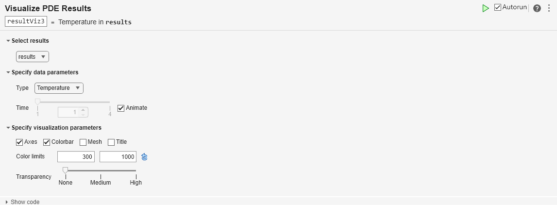
Animate the solution by selecting Animate. After the animation plays, the Live Editor displays the playback controls in the task window.

Click Show code to see and be able to copy the code used to create the plot. You can copy the generated code to recreate static and animated plots outside of the live script, and to modify and adapt the code to analyze different aspects of the problem or show results for a different problem. For example, copy the generated code that creates an animation and run it.

% Data to visualize
meshData2 = results.Mesh;
nodalData2 = results.Temperature(:,1);

% Create PDE result visualization
resultViz = pdeviz(meshData2,nodalData2, ...
    "ColorLimits",[300 1000]);
% Animate
figure
for ii2 = 1:4
    resultViz.NodalData = results.Temperature(:,ii2);
    pause(1.333)
end

You can also export the animation to a movie or an animated GIF file using the Export Animation button in the animation playback controls. For more information about creating animations in MATLAB®, see Animation Techniques.

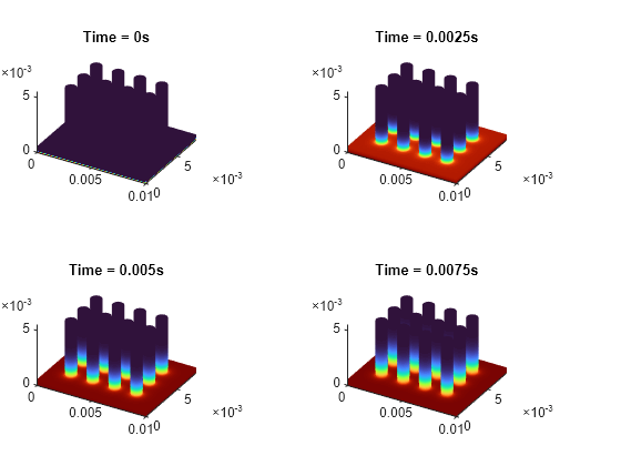
To show the temperatures for each time step next to each other, modify the generated code by using the tiledlayout function.

figure
t = tiledlayout(2,2,TileSpacing="tight", ...
                    Padding="none");
for ii2 = 1:4
    nexttile
    pdeviz(results.Mesh, ...
           results.Temperature(:,ii2), ...
           ColorbarVisible="off", ...
           Title={['Time = ' num2str(results.SolutionTimes(ii2)) 's']});
end