Optimize Green Hydrogen Production System

This example shows how to determine the key component sizes of a green system for producing hydrogen from an electrolyzer. The key components are as follows:

• Solar array

• Wind turbine

• Battery system

• Bidirectional connection to the electric grid

• Electrolyzer for producing hydrogen (H2)

• Electrical load

This figure illustrates how the various components are connected electrically.

Use techno-economic analysis to determine the optimal component sizes. The technical considerations include the physical and operational constraints of the green hydrogen production system. Assess the economic viability of investing in the system by using the net present value (NPV). Assume a 5% discount rate. Later in the example, you can examine the effect of different discount rates.

Problem Data

Load a data set consisting of hourly data over a 20-year period for the following:

• Load power (kW)

• Grid electricity price ($/kW)

• Solar profile (normalized to [0 1])

• Wind profile (normalized to [0 1])

• Green hydrogen price ($/kg)

In practice, this type of data might come from public or internal data sources, or from a predictive or forecasting model. For this example, load representative synthesized data into a single data structure (for convenience).

loadPower = load("loadPower.mat");
priceGrid = load("priceGrid.mat");
priceH2 = load("priceH2.mat");
solarProfile = load("solarProfile.mat");
windProfile = load("windProfile.mat");

data = struct(loadPower=loadPower.loadPower,...
    priceGrid=priceGrid.priceGrid,...
    priceH2=priceH2.priceH2,...
    solarProfile=solarProfile.solarProfile,...
    windProfile=windProfile.windProfile);

clear loadPower priceGrid priceH2 solarProfile windProfile

numYears = 20;
numSteps = 24*365*numYears; % Ignore the effects of leap years and seconds.
timeStep = 1; % unit = hours. Convert from power to energy by multiplying by timeStep.

For the NPV calculation, assume an annual discount rate of 5%.

discount_rate = 0.05;

Model Electric Consumption and Production

Model each component of the system. Begin by creating an optimization problem for maximization, where the objective is NPV (specified later in the example).

H2productionProblem = optimproblem(ObjectiveSense="maximize");

Treat all variables as continuous.

Grid Power

Create an optimization variable vector named gridPower representing the usage of grid power.

• Assume that the system can use up to 100 kW of power from the grid, and that the system can also supply up to 10 kW of power back to the grid. So, the system can both purchase power from the grid and sell power back to the grid.

• Assume that the price is the same for purchasing power from the grid and selling power back to the grid.

gridPowerBuyLimit = 100; % kW
gridPowerSellLimit = -10; % kW - negative value to indicate selling back to grid
gridPower = optimvar("gridPower",numSteps,...
    LowerBound=gridPowerSellLimit,UpperBound=gridPowerBuyLimit);

Solar Power

Create an optimization variable vector named solarRating representing the capacity of solar power.

• Assume a single solar unit whose maximum power is solarRating, where solarRating is an optimization variable no more than 500 kW.

• The hourly production of solar power is data.solarProfile*solarRating.

• The cost of the solar unit is directly proportional to its rating.

solarPowerCost = 1500; % $/kW of capacity, so total cost = solarPowerCost*solarRating.

The cost of the solar unit is taken from https://atb.nrel.gov/electricity/2021/residential_pv.

maxSolarRating = 500; % kW
solarRating = optimvar("solarRating",LowerBound=0,UpperBound=maxSolarRating);

Wind Power

Create an optimization variable vector named windRating representing the capacity of wind power.

• Assume a single wind unit whose maximum power is windRating, where windRating is an optimization variable no more than 500 kW.

• The hourly production of wind power is data.windProfile*windRating.

• The cost of the wind unit is directly proportional to its rating.

windPowerCost = 1500; % $/kW of capacity, so total cost = windPowerCost*windRating.
maxWindRating = 500; % kW
windRating = optimvar("windRating",LowerBound=0,UpperBound=maxWindRating);

Electric Storage

Model both power capacity (energy per unit of time in or out of storage) and total energy capacity.

• Assume that the power capacity is storagePowerRating, an optimization variable no more than 200 kW.

• Assume a single storage unit whose maximum energy capacity is storageEnergyRating, an optimization variable no more than 10,000 kWh.

The cost of a storage unit has three parts:

• Fixed cost of $5982

• Cost of $1690 per kW of power capacity

• Cost of $354 per kWh of energy capacity

These costs are taken from https://atb.nrel.gov/electricity/2021/residential_battery_storage.

storageFixedCost = 5982;   % $ one-time cost
storagePowerCost = 1690;   % $/kW
storageEnergyCost = 354;   % $/kWh

Create optimization variables for the storage unit. Create storagePower as a vector representing the power at each time step, and storageEnergy as a vector representing the energy at each time step. Also, create the scalar variables storagePowerRating and storageEnergyRating to represent the capacity of power and energy, respectively.

maxStoragePowerRating = 200; % kW
maxStorageEnergyRating = 10e3; % kWh
storagePower  = optimvar("storagePower",numSteps,...
    LowerBound=-maxStoragePowerRating,UpperBound=maxStoragePowerRating);
storageEnergy = optimvar("storageEnergy",numSteps,...
    LowerBound=0,UpperBound=maxStorageEnergyRating);
storagePowerRating = optimvar("storagePowerRating",LowerBound=0,UpperBound=maxStoragePowerRating);
storageEnergyRating = optimvar("storageEnergyRating",LowerBound=0,UpperBound=maxStorageEnergyRating);

The power and energy variables are related by energy balance: the power used or gained in an hour causes the energy stored to decrease or increase. Enforce this energy balance by creating optimization constraints.

storageEnergyBalance = optimconstr(numSteps); % Initialize
storageEnergyBalance(1) = storageEnergy(1) == -storagePower(1)*timeStep; % Initialize assuming zero stored energy at first
storageEnergyBalance(2:numSteps)   =  storageEnergy(2:numSteps) == ...
    storageEnergy(1:numSteps-1) - storagePower(2:numSteps)*timeStep;
H2productionProblem.Constraints.storageEnergyBalance = storageEnergyBalance;

The storage system degrades slowly over time. Model the storage system degradation by a 5% linear decline over the lifetime of the system for both storage capacity and power limits.

degradationFactor = linspace(1,1-0.05,numSteps)';
H2productionProblem.Constraints.chargeUpper = ...
    storageEnergy <= storageEnergyRating*degradationFactor;
H2productionProblem.Constraints.storagePowerLower1 = ...
    storagePower  >= -storagePowerRating*degradationFactor;
H2productionProblem.Constraints.storagePowerUpper = ...
    storagePower  <= storagePowerRating*degradationFactor;

Constrain the storage power to use only wind or solar power, not energy from the grid. This constraint ensures that the storage unit only supplies energy only from renewable sources during hydrogen production.

renewablePower = data.solarProfile*solarRating + data.windProfile*windRating;
H2productionProblem.Constraints.storagePowerLower2 = storagePower >= -renewablePower;

Electrolyzer Unit

Create an optimization variable named electrolyzerPower representing the power the electrolyzer uses at each hour, and an optimization variable named electrolyzerPowerRating representing the maximum for electrolyzerPower.

• Assume a single electrolyzer unit.

• The electrolyzer power rating can be between 0 and 50 kW.

• The electrolyzer produces hydrogen continuously and sells the stored hydrogen weekly.

• The cost for storing the hydrogen in the system is not considered.

• The electrolyzer uses 55 kWh of energy to produce 1 kg of hydrogen.

• The cost of the electrolyzer unit is proportional to its power capacity.

electrolyzerPowerCost = 4000; % $/kW of capacity, so total cost = electrolyzerPowerCost*electrolyzerPowerRating.

Create variables for the electrolyzer parameters.

maxElectrolyzerPowerRating = 50; % kW
H2SellInterval = 24*7; % hours in one week
H2ProdEnergy = 55; % kWh/kg

Create optimization variables for both the electrolyzer power and the stored hydrogen for each time step.

electrolyzerPower  = optimvar("electrolyzerPower",numSteps,...
    LowerBound=0,UpperBound=maxElectrolyzerPowerRating);
electrolyzerPowerRating = optimvar("electrolyzerPowerRating",LowerBound=0,UpperBound=maxElectrolyzerPowerRating);
H2_stored = optimvar("H2_stored",numSteps,LowerBound=0,UpperBound=1e12);

Create constraints enforcing the use of electrolyzer power to produce the hydrogen.

electrolyzerH2prod = optimconstr(numSteps);
electrolyzerH2prod(1) = H2_stored(1) == electrolyzerPower(1)*timeStep/H2ProdEnergy;
electrolyzerH2prod(2:numSteps) = H2_stored(2:numSteps) == ...
    H2_stored(1:numSteps-1) + electrolyzerPower(2:numSteps)*timeStep/H2ProdEnergy;
H2productionProblem.Constraints.electrolyzerH2prod = electrolyzerH2prod;

Create a constraint that all the produced hydrogen is sold at the specified intervals.

H2productionProblem.Constraints.electrolyzerH2prod(H2SellInterval+1:H2SellInterval:numSteps) = ...
    H2_stored(H2SellInterval+1:H2SellInterval:numSteps) == ...
    electrolyzerPower(H2SellInterval+1:H2SellInterval:numSteps)*timeStep/H2ProdEnergy;

Calculate how much hydrogen is sold at the specified selling intervals.

H2_sold = H2_stored(H2SellInterval:H2SellInterval:numSteps);

Constrain the electrolyzer power to maxElectrolyzerPowerRating, with linear degradation over time using the same degradation factor as for the storage unit power and energy capacity.

H2productionProblem.Constraints.electrolyzerPowerUpper1 = ...
    electrolyzerPower  <=  electrolyzerPowerRating*degradationFactor;

Constrain the electrolyzer to be supplied only by solar, wind, and storage power, not grid power. This constraint ensures that hydrogen is produced solely by renewable sources.

H2productionProblem.Constraints.electrolyzerPowerUpper2 = ...
    electrolyzerPower  <=  renewablePower + storagePower;

System Power Balance

Create a constraint that the power used plus the electrolyzer power is equal to the sum of the other power components.

H2productionProblem.Constraints.powerBalance = ...
    data.loadPower + electrolyzerPower == ... 
    gridPower + storagePower + ...
    data.solarProfile.*solarRating + ...
    data.windProfile.*windRating;

Create and Solve Optimization Problem

Summarize the costs of the system in a table.

Cost	Amount	Related Variable
Storage energy	$354/kWh	storageEnergyRating
Storage power	$1690/kW	storagePowerRating
Storage fixed	$5982 (one-time cost)	(none)
Solar power	$1500/kW	solarRating
Wind power	$1500/kW	windRating
Electrolyzer power	$4000/kW	electrolyzerPowerRating
Grid power	data.priceGrid	gridPower

Recall that NPV (net present value) is defined by

$$\mathrm{NPV}=\sum _{\mathit{t}=1}^{\mathit{N}}\frac{{\mathit{C}}_{\mathit{t}}}{{\left(1+\mathit{r}\right)}^{\mathit{t}}}-{\mathit{C}}_0,$$

where $\mathit{t}$ is a time period, $\mathit{N}$ is the total number of time periods, $\mathit{C}$ is cash flow, and $\mathit{r}$ is the discount rate.

Create an array of NPV correction factors to apply to each year's cash flow.

NPV_correction = 1./((1+discount_rate).^(1:20));

To apply the NPV correction at yearly intervals, calculate the annual cash flow from both purchasing power from the grid and selling power to the grid.

gridCashFlow = gridPower.*data.priceGrid;
gridCashFlowAnnual = sum(reshape(gridCashFlow,numYears,8760),2);

Similarly, calculate the cash flow from selling hydrogen. Because the sales interval for hydrogen is weekly instead of hourly, calculating the cash flow for each year is more complex.

priceH2_sellTimes = data.priceH2(H2SellInterval:H2SellInterval:numSteps);
H2cashFlow = H2_sold.*priceH2_sellTimes;

H2cashFlowAnnual = optimexpr(numYears,1);
j = 1; % year counter
for i = 1:size(H2cashFlow,1)
    if i > j*numSteps/(numYears*H2SellInterval)
        j = j + 1;
    end
    H2cashFlowAnnual(j,1) = H2cashFlowAnnual(j,1) + H2cashFlow(i,1);
end

Define the NPV expression, and set NPV as the objective function in the problem. Recall that the goal is to maximize the NPV.

NPV = dot(H2cashFlowAnnual,NPV_correction) - ...
      (dot(gridCashFlowAnnual,NPV_correction) + ...
      storageEnergyRating*storageEnergyCost + ...
      storagePowerRating*storagePowerCost + ...
      storageFixedCost + ...
      solarRating*solarPowerCost + ...
      windRating*windPowerCost + ...
      electrolyzerPowerRating*electrolyzerPowerCost);
H2productionProblem.Objective = NPV;

To solve an optimization problem you call the solve function. solve automatically selects an appropriate solver from the problem definition. To set options for solve, find out which solver is default for this problem.

defaultSolver = solvers(H2productionProblem)

defaultSolver = 
"linprog"

Next, set options so the linprog solver uses the "interior-point" algorithm, which is typically efficient on large problems. To monitor the solver during the lengthy solution process, specify the iterative display.

opt = optimoptions("linprog",Display="iter",Algorithm="interior-point");

Call solve, timing the solution process.

tic
[sol,fval,exitflag,output] = solve(H2productionProblem,Options=opt);

Solving problem using linprog.

LP preprocessing removed 0 inequalities, 350399 equalities,
350399 variables, and 174159 non-zero elements.

 Iter            Fval  Primal Infeas    Dual Infeas  Complementarity  
    0   -1.178573e+06   5.608917e+07   5.929097e+03     2.964549e+03  
    1   -1.294799e+06   4.782009e+07   5.074830e+03     2.441886e+03  
    2   -1.216946e+06   4.740283e+07   5.026792e+03     2.414537e+03  
    3   -1.266976e+06   4.498470e+07   4.802786e+03     2.268036e+03  
    4   -1.344059e+06   4.148931e+07   4.418628e+03     2.040061e+03  
    5   -1.459946e+06   3.672841e+07   3.922874e+03     1.769770e+03  
    6   -1.598636e+06   3.129757e+07   3.342334e+03     1.480302e+03  
    7   -1.785361e+06   2.428260e+07   2.602958e+03     1.227211e+03  
    8   -1.916342e+06   1.958880e+07   2.012040e+03     1.093408e+03  
    9   -1.689461e+06   1.751712e+07   1.393381e+03     8.358795e+02  
   10   -1.957988e+06   4.080368e+06   6.692198e+02     2.933479e+02  
   11   -1.988372e+06   1.747661e+06   1.585078e+02     2.550027e+02  
   12   -1.998031e+06   1.090897e+06   7.118769e+01     2.486920e+02  
   13   -2.015560e+06   5.454483e+02   1.312017e+01     2.205156e+02  
   14   -1.472100e+06   2.727241e-01   1.133669e+00     2.243413e+02  
   15   -1.247088e+06   2.327862e-01   4.467992e-01     2.227040e+02  
   16   -1.011834e+06   1.870706e-01   4.059827e-01     1.967737e+02  
   17   -3.995249e+05   9.608554e-02   2.486819e-01     1.956419e+02  
   18   -2.423202e+05   7.614850e-02   1.566068e-01     1.995608e+02  
   19   -2.551991e+05   7.501003e-02   1.565408e-01     2.035987e+02  
   20   -1.974084e+05   6.142701e-02   1.046904e-01     2.131338e+02  
   21   -1.460593e+05   5.114859e-02   8.894056e-02     2.031718e+02  
   22   -2.336601e+04   3.434271e-02   5.155711e-02     2.323979e+02  
   23   -1.317895e+04   2.657238e-02   4.235897e-02     2.091003e+02  
   24    4.224243e+04   1.914868e-02   3.588444e-02     1.783931e+02  
   25    9.458115e+04   1.268196e-02   2.059030e-02     1.067190e+02  
   26    1.146454e+05   1.047946e-02   1.624021e-02     8.518709e+01  
   27    1.372382e+05   8.093186e-03   1.484747e-02     7.817832e+01  
   28    1.465847e+05   6.957344e-03   1.479635e-02     7.790480e+01  
   29    1.487576e+05   6.967015e-03   1.442592e-02     7.602382e+01  
 Iter            Fval  Primal Infeas    Dual Infeas  Complementarity  
   30    1.676377e+05   4.945382e-03   1.292945e-02     6.839695e+01  
   31    1.795370e+05   3.359460e-03   1.243312e-02     6.580424e+01  
   32    1.931510e+05   2.236006e-03   7.443035e-03     3.988819e+01  
   33    1.993582e+05   1.709777e-03   6.742025e-03     3.618831e+01  
   34    2.048188e+05   1.272149e-03   4.943141e-03     2.670239e+01  
   35    2.071359e+05   1.049014e-03   4.469862e-03     2.444963e+01  
   36    2.094030e+05   9.004983e-04   3.935627e-03     2.190758e+01  
   37    2.139528e+05   6.237723e-04   2.859281e-03     2.139605e+01  
   38    2.162734e+05   4.970542e-04   2.775039e-03     2.118995e+01  
   39    2.165535e+05   4.818491e-04   2.428397e-03     2.116179e+01  
   40    2.183957e+05   3.870436e-04   1.946604e-03     2.100559e+01  
   41    2.202637e+05   2.976011e-04   1.579697e-03     2.079664e+01  
   42    2.204660e+05   2.731233e-04   1.424365e-03     1.976317e+01  
   43    2.216065e+05   2.189203e-04   8.068814e-04     1.146913e+01  
   44    2.236125e+05   1.414639e-04   5.012256e-04     7.184765e+00  
   45    2.245949e+05   1.080341e-04   3.191582e-04     4.596675e+00  
   46    2.253382e+05   8.502100e-05   2.620995e-04     3.779332e+00  
   47    2.256644e+05   7.534886e-05   1.768031e-04     2.554394e+00  
   48    2.269214e+05   4.077266e-05   3.614674e-04     1.388137e+00  
   49    2.277130e+05   2.099447e-05   2.122922e-04     8.154364e-01  
   50    2.281012e+05   1.222097e-05   9.001300e-05     3.460406e-01  
   51    2.284216e+05   5.980359e-06   3.637304e-05     1.394308e-01  
   52    2.286027e+05   2.941528e-06   1.763476e-05     6.747154e-02  
   53    2.286935e+05   1.593924e-06   8.537766e-06     3.268591e-02  
   54    2.287549e+05   7.964201e-07   2.335121e-05     1.623783e-02  
   55    2.287552e+05   7.909396e-07   4.826724e-04     3.072584e-02  
   56    2.287851e+05   4.517309e-07   3.114561e-04     2.143220e-02  
   57    2.288086e+05   2.107679e-07   8.339936e-05     1.404208e-02  
   58    2.288222e+05   9.975881e-08   4.899503e-05     1.272611e-02  
   59    2.288293e+05   4.793552e-08   2.250390e-05     1.438920e-02  
 Iter            Fval  Primal Infeas    Dual Infeas  Complementarity  
   60    2.288362e+05   3.834084e-04   5.365681e-06     8.763467e-03  
   61    2.288374e+05   2.106285e-04   7.856177e-06     4.767058e-03  
   62    2.288392e+05   1.983401e-06   1.438787e-06     3.903828e-05  
   63    2.288392e+05   2.306187e-04   5.429682e-08     9.674544e-08  

Minimum found that satisfies the constraints.

Optimization completed because the objective function is non-decreasing in feasible directions, to within the function tolerance, and constraints are satisfied to within the constraint tolerance.

toc

Elapsed time is 624.731417 seconds.

Analyze Results

Show the optimized NPV.

optimizedNPV = fval

optimizedNPV = 
2.2884e+05

Because the NPV is positive, the project is economically worthwhile.

Extract the optimization solution values for analysis.

solarPowerVal              = data.solarProfile*sol.solarRating;
solarPowerRatingVal             = sol.solarRating;
windPowerVal               = data.windProfile*sol.windRating;
windPowerRatingVal         = sol.windRating;
gridPowerVal               = sol.gridPower;
storagePowerVal            = sol.storagePower;
storagePowerRatingVal      = sol.storagePowerRating;
storageEnergyRatingVal     = sol.storageEnergyRating;
electrolyzerPowerVal       = sol.electrolyzerPower;
electrolyzerPowerRatingVal = sol.electrolyzerPowerRating;

Create a table to display the solution variables.

systemComponents = ["Solar Power Rating (kW)";"Wind Power Rating (kW)"; ...
    "Storage Power Rating (kW)";"Storage Energy Rating (kWh)"; ...
    "Electrolyzer Power Rating (kW)"];
lowerBounds = zeros(5,1);
upperBounds = [maxSolarRating; maxWindRating; maxStoragePowerRating;...
    maxStorageEnergyRating; maxElectrolyzerPowerRating];
optimizedRatings = [solarPowerRatingVal; windPowerRatingVal; storagePowerRatingVal; ...
    storageEnergyRatingVal; electrolyzerPowerRatingVal];

resultsTable = table(systemComponents,lowerBounds,upperBounds,optimizedRatings)

resultsTable=5×4 table
            systemComponents            lowerBounds    upperBounds    optimizedRatings
    ________________________________    ___________    ___________    ________________

    "Solar Power Rating (kW)"                0              500            42.216     
    "Wind Power Rating (kW)"                 0              500            114.54     
    "Storage Power Rating (kW)"              0              200            37.688     
    "Storage Energy Rating (kWh)"            0            10000            199.02     
    "Electrolyzer Power Rating (kW)"         0               50                50     

The optimal electrolyzer power rating is at its upper bound of 50. This result suggests that using an electrolyzer with a rating larger than 50 kW might produce a higher NPV for the project.

Examine System Operations

Examine the operation of the system in detail. First, create a time vector for the 20-year period.

t1 = datetime(2024,1,1,0,0,0);
t2 = datetime(2024 + numYears - 1,12,31,23,0,0);
t = linspace(t1,t2,numSteps);

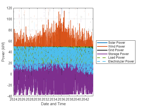
Plot the time series data of solar power, wind power, grid power, storage power, load power, and electrolyzer power.

figure
p = plot(t,solarPowerVal,t,windPowerVal,t,gridPowerVal,"k",t,storagePowerVal,t, ...
    data.loadPower,"--",t,electrolyzerPowerVal,"--",LineWidth=2);
grid
legend("Solar Power","Wind Power","Grid Power","Storage Power","Load Power","Electrolyzer Power",Location="eastoutside")
xlabel("Date and Time"),ylabel("Power (kW)")

To see the curves in more detail, zoom in to view a one-week period.

xlim([t(1e3),t(1e3+24*7)])

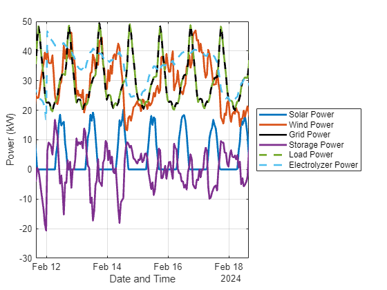
The level of detail reveals the following:

• The grid power and load power curves are identical. For this time range, the load is fully supplied by the grid.

• Storage power tends to become negative as solar power nears its maximum. The battery system tends to store some solar energy when solar power is available, and supplies power when solar power is not available.

• Electrolyzer power is correlated with wind power, but is not identical.

Plot the grid power and grid price profile.

figure
plot(t,sol.gridPower,"k");
xlabel("Date and Time"),ylabel("Grid Power (kW)")
grid
hold on
yyaxis right
plot(t,data.priceGrid);
ylabel("Grid Power Price ($/kW)")
ylim([min(data.priceGrid) max(data.priceGrid)])
hold off

Zoom in for a closer look.

xlim([t(1e5) t(1.002e5)])

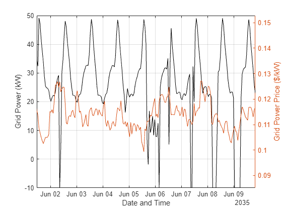
• Grid power sometimes becomes negative, indicating power being sold back to the grid.

• Power is typically sold back to the grid when the grid price is higher, but not always. This result highlights the value of using optimization when making decisions in this type of complex problem.

Calculate and plot the cumulative hydrogen sold.

H2_sold_cum = cumsum(sol.H2_stored);
totalH2 = H2_sold_cum(end);
fprintf("Total H2 sold in kg: %g\n",totalH2)

Total H2 sold in kg: 1.09691e+07

figure
plot(t,H2_sold_cum);
xlabel("Date and Time")
ylabel("Cumulative Hydrogen Sold (kg)")
grid

The cumulative hydrogen sold is linearly increasing in time (roughly).

Plot the stored hydrogen profile over a four-week period. Note that stored hydrogen increases throughout the week, and then drops at the end of the week when it is sold.

figure
plot(t,sol.H2_stored);
xlabel("Date and Time")
ylabel("Stored Hydrogen (kg)")
xlim([t(1e3),t(1e3+24*7*4)])
grid

Change Discount Rate

What is the effect of the discount rate on the economics of this system? Calculate the results for a range of discount rates. This calculation takes a long time, so use parallel computing if it is available.

nrates = 16;
discountRate = linspace(.02,.08,nrates);
% Create arrays to hold the results.
sols = cell(nrates,1);
fvals = zeros(1,nrates);
opt.Display = "none";
allconstraints = H2productionProblem.Constraints;
tic
parfor i = 1:nrates
    NPVCorrection = 1./((1+discountRate(i)).^(1:numYears));
    NPV = dot(H2cashFlowAnnual,NPVCorrection) - ...
        (dot(gridCashFlowAnnual,NPVCorrection) + ...
        storageEnergyRating*storageEnergyCost + ...
        storagePowerRating*storagePowerCost + ...
        storageFixedCost + ...
        solarRating*solarPowerCost + ...
        windRating*windPowerCost + ...
        electrolyzerPowerRating*electrolyzerPowerCost);
    H2productionProblem = optimproblem(Objective=NPV,...
        Constraints=allconstraints,ObjectiveSense="max");
    [tempsol,tempfval] = solve(H2productionProblem,Options=opt);
    sols{i} = tempsol;
    fvals(i) = tempfval;
end
toc

Elapsed time is 3340.941009 seconds.

Plot the NPV as a function of the discount rate.

figure
plot(discountRate,fvals,"bo")
xlabel("Discount Rate")
ylabel("NPV")

The optimal NPV decreases smoothly from 5e5 to 7e4 as the discount rate increases from 2% to 8%. The optimal curve appears to be convex, which implies that the NPV is more sensitive to changes in the discount rate when it is small and is less sensitive when it is large.

Plot how the optimal solar, wind, storage, and electrolyzer ratings respond to different discount rates.

solarPowerRatings = zeros(1,nrates);
windPowerRatings = zeros(1,nrates);
storagePowerRatings = zeros(1,nrates);
storageEnergyRatings = zeros(1,nrates);
electrolyzerPowerRatings = zeros(1,nrates);
Total_H2_Sold = zeros(1,nrates);
for i = 1:nrates
    solarPowerRatings(i) = sols{i}.solarRating;
    windPowerRatings(i) = sols{i}.windRating;
    storagePowerRatings(i) = sols{i}.storagePowerRating;
    storageEnergyRatings(i) = sols{i}.storageEnergyRating;
    electrolyzerPowerRatings(i) = sols{i}.electrolyzerPowerRating;
    Total_H2_Sold(i) = sum(sols{i}.H2_stored);
end
figure
tiledlayout(3,2,TileSpacing="tight")
nexttile
plot(discountRate,solarPowerRatings,"bo")
xlabel("Discount Rate")
ylabel("Solar Power")
nexttile
plot(discountRate,windPowerRatings,"bo")
xlabel("Discount Rate")
ylabel("Wind Power")
nexttile
plot(discountRate,storagePowerRatings,"bo")
xlabel("Discount Rate")
ylabel("Storage Power")
nexttile
plot(discountRate,storageEnergyRatings,"bo")
xlabel("Discount Rate")
ylabel("Storage Energy")
nexttile
plot(discountRate,electrolyzerPowerRatings,"bo")
xlabel("Discount Rate")
ylabel("Electrolyzer Power")
ylim([49 50])
nexttile
plot(discountRate,Total_H2_Sold,"bo")
xlabel("Discount Rate")
ylabel("Total H2 Sold")

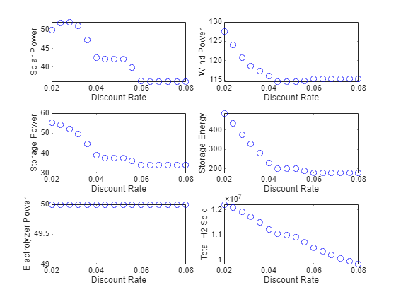
• The solar power rating is not a monotone function of the discount rate. The highest observed optimal solar power rating is about 52 kW, and the smallest is about 36 kW.

• Similarly, the wind rating does not have a monotone response to the discount rate. The highest observed wind power rating is almost 128 kW, and the lowest is a bit over 114 kW.

• The storage power rating is nonincreasing. The highest observed storage power rating is 55 kW, and the lowest is 34 kW.

• Similarly, the storage energy rating is nonincreasing. The highest observed storage energy rating is near 500 kWh, and the lowest is just under 200 kWh.

• The optimal electrolyzer power rating is 50 kW for all discount rates. This result implies that you can improve the NPV by using a higher electrolyzer power rating.

• The total hydrogen sold over the 20-year period is monotone decreasing in the discount rate, and is neither concave nor convex. The highest observed amount of hydrogen sold is over 1.2e7 kg, and the lowest is just under 1e7 kg.

Conclusion

The analysis of the green hydrogen production system shows that the system is economical to use for all discount rates between 2% and 8%. The operational details of the system show some unexpected variations in response to different discount rates. Specifically, the system component ratings are not strictly monotone functions of the discount rate. The optimal solutions include hourly settings for the various system components, as shown in the section Examine System Operations.