checkGradients

Check first derivative function against finite-difference approximation

Since R2023b

Syntax

valid = checkGradients(fun,x0)

valid = checkGradients(fun,x0,options)

valid = checkGradients(___,Name=Value)

[valid,err] = checkGradients(___)

Description

valid = checkGradients(fun,x0) compares the value of the supplied first derivative function in fun at a point near x0 against a finite-difference approximation. By default, the comparison assumes that the function is an objective function. To check constraint functions, set the IsConstraint name-value argument to true.

valid = checkGradients(fun,x0,options) modifies the comparison by changing finite differencing options.

valid = checkGradients(___,Name=Value) specifies additional options using one or more name-value arguments, in addition to any of the input argument combinations in the previous syntaxes. For example, you can set the tolerance for the comparison, or specify that the comparison is for nonlinear constraint functions.

[valid,err] = checkGradients(___) also returns a structure err containing the relative differences between the supplied derivatives and finite-difference approximations.

Examples

Check Objective Gradient

The rosen function at the end of this example computes the Rosenbrock objective function and its gradient for a 2-D variable x.

Check that the computed gradient in rosen matches a finite-difference approximation near the point [2,4].

x0 = [2,4];
valid = checkGradients(@rosen,x0)

valid = logical
   1

function [f,g] = rosen(x)
f = 100*(x(1) - x(2)^2)^2 + (1 - x(2))^2;
if nargout > 1
    g(1) = 200*(x(1) - x(2)^2);
    g(2) = -400*x(2)*(x(1) - x(2)^2) - 2*(1 - x(2));
end
end

Check Least-Squares Objective Gradient

The vecrosen function at the end of this example computes the Rosenbrock objective function in least-squares form and its Jacobian (gradient).

Check that the computed gradient in vecrosen matches a finite-difference approximation near the point [2,4].

x0 = [2,4];
valid = checkGradients(@vecrosen,x0)

valid = logical
   1

function [f,g] = vecrosen(x)
f = [10*(x(1) - x(2)^2),1-x(1)];
if nargout > 1
    g = zeros(2); % Allocate g
    g(1,1) = 10; % df(1)/dx(1)
    g(1,2) = -20*x(2); % df(1)/dx(2)
    g(2,1) = -1; % df(2)/dx(1)
    g(2,2) = 0; % df(2)/dx(2)
end
end

Modify Finite-Difference Options

The rosen function at the end of this example computes the Rosenbrock objective function and its gradient for a 2-D variable x.

For some initial points, the default forward finite differences cause checkGradients to mistakenly indicate that the rosen function has incorrect gradients. To see result details, set the Display option to "on".

x0 = [0,0];
valid = checkGradients(@rosen,x0,Display="on")

____________________________________________________________

Objective function derivatives:
Maximum relative difference between supplied 
and finite-difference derivatives = 1.48826e-06.
  Supplied derivative element (1,1): -0.126021
  Finite-difference derivative element (1,1): -0.126023

checkGradients failed.

Supplied derivative and finite-difference approximation are
not within 'Tolerance' (1e-06).
____________________________________________________________

valid = logical
   0

checkGradients reports a mismatch, with a difference of just over 1 in the sixth decimal place. Use central finite differences and check again.

opts = optimoptions("fmincon",FiniteDifferenceType="central");
valid = checkGradients(@rosen,x0,opts,Display="on")

____________________________________________________________

Objective function derivatives:
Maximum relative difference between supplied 
and finite-difference derivatives = 1.29339e-11.

checkGradients successfully passed.
____________________________________________________________

valid = logical
   1

Central finite differences are generally more accurate. checkGradients reports that the gradient and central finite-difference approximation match to about 11 decimal places.

function [f,g] = rosen(x)
f = 100*(x(1) - x(2)^2)^2 + (1 - x(2))^2;
if nargout > 1
    g(1) = 200*(x(1) - x(2)^2);
    g(2) = -400*x(2)*(x(1) - x(2)^2) - 2*(1 - x(2));
end
end

Check Gradients of Nonlinear Constraints

The tiltellipse function at the end of this example imposes the constraint that the 2-D variable x is confined to the interior of the tilted ellipse

$$\frac{xy}{2}+(x+2{)}^2+\frac{(y-2{)}^2}{2}\le 2$$.

Visualize the ellipse.

f = @(x,y) x.*y/2+(x+2).^2+(y-2).^2/2-2;
fcontour(f,LevelList=0)
axis([-6 0 -1 7])

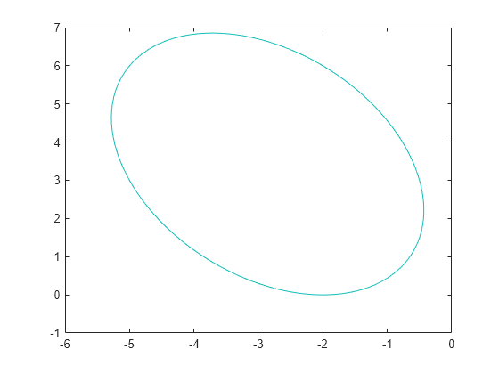
Check the gradient of this nonlinear inequality constraint function.

x0 = [-2,6];
valid = checkGradients(@tiltellipse,x0,IsConstraint=true)

valid = 1×2 logical array

   1   1

function [c,ceq,gc,gceq] = tiltellipse(x)
c = x(1)*x(2)/2 + (x(1) + 2)^2 + (x(2)- 2)^2/2 - 2;
ceq = [];

if nargout > 2
   gc = [x(2)/2 + 2*(x(1) + 2);
       x(1)/2 + x(2) - 2];
   gceq = [];
end
end

Examine Differences Between Gradients and Finite-Difference Approximations

The fungrad function at the end of this example correctly calculates the gradient of some components of the least-squares objective, and incorrectly calculates others.

Examine the second output of checkGradients to see which components do not match well at the point [2,4]. To see result details, set the Display option to "on".

x0 = [2,4];
[valid,err] = checkGradients(@fungrad,x0,Display="on")

____________________________________________________________

Objective function derivatives:
Maximum relative difference between supplied 
and finite-difference derivatives = 0.749797.
  Supplied derivative element (3,2): 19.9838
  Finite-difference derivative element (3,2): 5

checkGradients failed.

Supplied derivative and finite-difference approximation are
not within 'Tolerance' (1e-06).
____________________________________________________________

valid = logical
   0

err = struct with fields:
    Objective: [3×2 double]

The output shows that element [3,2] is incorrect. But is that the only problem? Examine err.Objective and look for entries that are far from 0.

err.Objective

ans = 3×2

    0.0000    0.0000
    0.0000         0
    0.5000    0.7498

Both the [3,1] and [3,2] elements of the derivative are incorrect. The fungrad2 function at the end of this example corrects the errors.

[valid,err] = checkGradients(@fungrad2,x0,Display="on")

____________________________________________________________

Objective function derivatives:
Maximum relative difference between supplied 
and finite-difference derivatives = 2.2338e-08.

checkGradients successfully passed.
____________________________________________________________

valid = logical
   1

err = struct with fields:
    Objective: [3×2 double]

err.Objective

ans = 3×2
10-7 ×

    0.2234    0.0509
    0.0003         0
    0.0981    0.0042

All the differences between the gradient and finite-difference approximations are less than 1e-7 in magnitude.

This code creates the fungrad helper function.

function [f,g] = fungrad(x)
f = [10*(x(1) - x(2)^2),1 - x(1),5*(x(2) - x(1)^2)];

if nargout > 1
    g = zeros(3,2);
    g(1,1) = 10;
    g(1,2) = -20*x(2);
    g(2,1) = -1;
    g(3,1) = -20*x(1);
    g(3,2) = 5*x(2);
end
end

This code creates the fungrad2 helper function.

function [f,g] = fungrad2(x)
f = [10*(x(1) - x(2)^2),1 - x(1),5*(x(2) - x(1)^2)];

if nargout > 1
    g = zeros(3,2);
    g(1,1) = 10;
    g(1,2) = -20*x(2);
    g(2,1) = -1;
    g(3,1) = -10*x(1);
    g(3,2) = 5;
end
end

Check lsqcurvefit Gradient

When you provide gradient evaluation functions, nonlinear least-squares solvers such as lsqcurvefit can run faster and more reliably. However, the lsqcurvefit solver has a slightly different syntax for checking gradients compared to other solvers.

Fitting Problem and checkGradient Syntax

To check an lsqcurvefit gradient, instead of passing in the initial point x0 as an array, pass the cell array {x0,xdata}. For example, for the response function $$y=a+b\exp (-cx)$$, create data ydata from the model with added noise. The response function is fitfun.

function [F,J] = fitfun(x,xdata)
F = x(1) + x(2)*exp(-x(3)*xdata);
if nargout > 1
    J = [ones(size(xdata)) exp(-x(3)*xdata) -xdata.*x(2).*exp(-x(3)*xdata)];
end
end

Create xdata as random points from 0 to 10, and ydata as the response plus added noise.

a = 2;
b = 5;
c = 1/15;
N = 100;
rng default
xdata = 10*rand(N,1);
fun = @fitfun;
ydata = fun([a,b,c],xdata) + randn(N,1)/10;

Check that the gradient of the response function is correct at the point [a,b,c].

[valid,err] = checkGradients(@fitfun,{[a b c] xdata})

valid = logical
   1

err = struct with fields:
    Objective: [100×3 double]

You can safely use the provided objective gradient. Set the lower bound of all parameters to 0, with no upper bound.

options = optimoptions("lsqcurvefit",SpecifyObjectiveGradient=true);
lb = zeros(1,3);
ub = [];
[sol,res,~,eflag,output] = lsqcurvefit(fun,[1 2 1],xdata,ydata,lb,ub,options)

Local minimum possible.

lsqcurvefit stopped because the final change in the sum of squares relative to 
its initial value is less than the value of the function tolerance.

<stopping criteria details>

sol = 1×3

    2.5872    4.4376    0.0802

res = 
1.0096

eflag = 
3

output = struct with fields:
      firstorderopt: 4.4156e-06
         iterations: 25
          funcCount: 26
       cgiterations: 0
          algorithm: 'trust-region-reflective'
           stepsize: 1.8029e-04
            message: 'Local minimum possible.↵↵lsqcurvefit stopped because the final change in the sum of squares relative to ↵its initial value is less than the value of the function tolerance.↵↵<stopping criteria details>↵↵Optimization stopped because the relative sum of squares (r) is changing↵by less than options.FunctionTolerance = 1.000000e-06.'
       bestfeasible: []
    constrviolation: []

Nonlinear Constraint Function in lsqcurvefit

The required syntax for nonlinear constraint functions differs from the syntax of the lsqcurvefit objective function. A nonlinear constraint function with gradient has this form:

function [c,ceq,gc,gceq] = ccon(x)
c = ...
ceq = ...
if nargout > 2
    gc = ...
    gceq = ...
end
end

The gradient expressions must be of size N-by-Nc, where N is the number of problem variables, and Nc is the number of constraint functions. For example, the ccon function below has just one nonlinear inequality constraint. So, the function returns a gradient of size 3-by-1 for this problem with three variables.

function [c,ceq,gc,gceq] = ccon(x)
ceq = [];
c = x(1)^2 + x(2)^2 + 1/x(3)^2 - 50;
if nargout > 2
    gceq = [];
    gc = zeros(3,1); % Gradient is a column vector
    gc(1) = 2*x(1);
    gc(2) = 2*x(2);
    gc(3) = -2/x(3)^3;
end
end

Check whether the ccon function returns a correct gradient at the point [a,b,c].

[valid,err] = checkGradients(@ccon,[a b c],IsConstraint=true)

valid = 1×2 logical array

   1   1

err = struct with fields:
    Inequality: [3×1 double]
      Equality: []

To use the constraint gradient, set options to use the gradient function, and then solve the problem again with the nonlinear constraint.

options.SpecifyConstraintGradient = true;
[sol2,res2,~,eflag2,output2] = lsqcurvefit(@fitfun,[1 2 1],xdata,ydata,lb,ub,[],[],[],[],@ccon,options)

Local minimum found that satisfies the constraints.

Optimization completed because the objective function is non-decreasing in 
feasible directions, to within the value of the optimality tolerance,
and constraints are satisfied to within the value of the constraint tolerance.

<stopping criteria details>

sol2 = 1×3

    4.4436    2.8548    0.2127

res2 = 
2.2623

eflag2 = 
1

output2 = struct with fields:
         iterations: 15
          funcCount: 22
    constrviolation: 0
           stepsize: 1.7914e-06
          algorithm: 'interior-point'
      firstorderopt: 3.3350e-06
       cgiterations: 0
            message: 'Local minimum found that satisfies the constraints.↵↵Optimization completed because the objective function is non-decreasing in ↵feasible directions, to within the value of the optimality tolerance,↵and constraints are satisfied to within the value of the constraint tolerance.↵↵<stopping criteria details>↵↵Optimization completed: The relative first-order optimality measure, 1.621619e-07,↵is less than options.OptimalityTolerance = 1.000000e-06, and the relative maximum constraint↵violation, 0.000000e+00, is less than options.ConstraintTolerance = 1.000000e-06.'
       bestfeasible: [1×1 struct]

The residual res2 is more than twice as large as the residual res, which has no nonlinear constraint. This result suggests that the nonlinear constraint keeps the solution away from the unconstrained minimum.

Plot the solution with and without the nonlinear constraint.

scatter(xdata,ydata)
hold on
scatter(xdata,fitfun(sol,xdata),"x")
hold off
xlabel("x")
ylabel("y")
legend("Data","Fitted")
title("Data and Fitted Response, No Constraint")

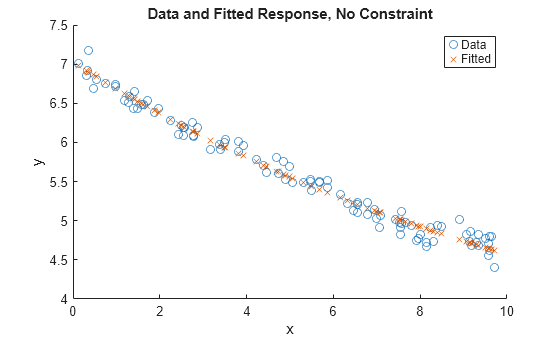
figure
scatter(xdata,ydata)
hold on
scatter(xdata,fitfun(sol2,xdata),"x")
hold off
xlabel("x")
ylabel("y")
legend("Data","Fitted with Constraint")
title("Data and Fitted Response with Constraint")

Input Arguments

fun — Function to check

function handle

Function to check, specified as a function handle.

• If fun represents an objective function, then fun must have the following signature.

  [fval,grad] = fun(x)

  checkGradients compares the value of grad(x) to a finite-difference approximation for a point x near x0. The comparison is

  $$\left|\frac{\text{grad}\_\text{fd }-\text{ grad}}{\text{max}\left(\text{1},\left|\text{grad}\right|\right)}\right|,$$

  where grad represents the value of the gradient function, and grad_fd represents the value of the finite-difference approximation. checkGradients performs this division component-wise.

• If fun represents a least-squares objective, then fun is a vector, and grad(x) is a matrix representing the Jacobian of fun.

  If fun returns an array of m components and x has n elements, where n is the number of elements of x0, the Jacobian J is an m-by-n matrix where J(i,j) is the partial derivative of F(i) with respect to x(j). (The Jacobian J is the transpose of the gradient of F.)

• If fun represents a nonlinear constraint, then fun must have the following signature.

  [c,ceq,gc,gceq] = fun(x)

  • c represents the nonlinear inequality constraints. Solvers attempt to achieve c <= 0. The c output can be a vector of any length.

  • ceq represents the nonlinear equality constraints. Solvers attempt to achieve ceq = 0. The ceq output can be a vector of any length.

  • gc represents the gradient of the nonlinear inequality constraints. Your gradient should be of size N-by-Nc, where N is the number of problem variables, and Nc is the number of elements of c.

  • gceq represents the gradient of the nonlinear equality constraints. Your gradient should be of size N-by-Nceq, where N is the number of problem variables, and Nceq is the number of elements of ceq.

Data Types: function_handle

x0 — Location to check gradient

double array | 1-by-2 cell array

Location at which to check the gradient, specified as a double array for all solvers except lsqcurvefit. For lsqcurvefit, x0 is a 1-by-2 cell array {x0array,xdata}.

checkGradients checks the gradient at a point near the specified x0. The function adds a small random direction to x0, no more than 1e-3 in absolute value. This perturbation attempts to protect the check against a point where an incorrect gradient function might pass because of cancellations.

Example: randn(5,1)

Data Types: double
Complex Number Support: Yes

options — Finite differencing options

output of optimoptions

Finite differencing options, specified as the output of optimoptions. The following options affect finite differencing.

Option	Description
FiniteDifferenceStepSize	Scalar or vector step size factor for finite differences. When you set FiniteDifferenceStepSize to a vector v, the forward finite differences delta are delta = v.*sign′(x).*max(abs(x),TypicalX); where sign′(x) = sign(x) except sign′(0) = 1. Central finite differences are delta = v.*max(abs(x),TypicalX); A scalar FiniteDifferenceStepSize expands to a vector. The default is sqrt(eps) for forward finite differences, and eps^(1/3) for central finite differences.
FiniteDifferenceType	Finite differences used to estimate gradients are either "forward" (default), or "central" (centered). "central" takes twice as many function evaluations but is usually more accurate.
TypicalX	Typical x values. The number of elements in TypicalX is equal to the number of elements in the starting point x0. The default value is ones(numberofvariables,1).
DiffMaxChange (discouraged)	Maximum change in variables for finite-difference gradients (a positive scalar). The default is Inf.
DiffMinChange (discouraged)	Minimum change in variables for finite-difference gradients (a nonnegative scalar). The default is 0.

Example: optimoptions("fmincon",FiniteDifferenceStepSize=1e-4)

Name-Value Arguments

Specify optional pairs of arguments as Name1=Value1,...,NameN=ValueN, where Name is the argument name and Value is the corresponding value. Name-value arguments must appear after other arguments, but the order of the pairs does not matter.

Before R2021a, use commas to separate each name and value, and enclose Name in quotes.

Example: IsConstraint=true,Tolerance=5e-4

Display — Flag to display results at command line

"off" (default) | "on"

Flag to display results at command line, specified as "off" (do not display the results) or "on" (display the results).

Example: "off"

Data Types: char | string

IsConstraint — Flag to check nonlinear constraint gradients

false (default) | true

Flag to check nonlinear constraint gradients, specified as false (the function is an objective function) or true (the function is a nonlinear constraint function).

Example: true

Data Types: logical

Tolerance — Tolerance for gradient approximation

1e-6 (default) | nonnegative scalar

Tolerance for the gradient approximation, specified as a nonnegative scalar. The returned value valid is true for each component where the absolute relative difference between the gradient of fun and its finite-difference approximation is less than or equal to Tolerance.

Example: 1e-3

Data Types: double

Output Arguments

valid — Indication that finite-difference approximation matches gradient

logical scalar | two-element logical vector

Indication that the finite-difference approximation matches the gradient, returned as a logical scalar for objective functions or a two-element logical vector for nonlinear constraint functions [c,ceq]. The returned value valid is true when the absolute relative difference between the gradient of fun and its finite-difference approximation is less than or equal to Tolerance for all components of the gradient. Otherwise, valid is false.

When a nonlinear constraint c or ceq is empty, the returned value of valid for that constraint is true.

err — Relative differences between gradients and finite-difference approximations

structure

Relative differences between the gradients and finite-difference approximations, returned as a structure. For objective functions, the field name is Objective. For nonlinear constraint functions, the field names are Inequality (corresponding to c) and Equality (corresponding to ceq). Each component of err has the same shape as the supplied derivatives from fun.

More About

CheckGradients Failed

Gradients or Jacobians estimated near the initial point did not match the supplied derivatives to within a default tolerance of 1e-6 or, for the checkGradients function, the specified Tolerance value.

• Usually, this failure means that your objective or nonlinear constraint functions have an incorrect derivative calculation. Double-check the indicated derivative.

• Occasionally, the finite difference approximations to the derivatives are inaccurate enough to cause the failure. This inaccuracy can occur when the second derivative of a function (objective or nonlinear constraint) has a large magnitude. It can also occur when using the default 'forward' finite differences, which are less accurate but faster than 'central' finite differences. If you think that the derivative functions are correct, try one or both of the following to see if CheckGradients passes:

  • Set the FiniteDifferenceType option to 'central'.

  • Set the FiniteDifferenceStepSize option to a small value such as 1e-10.

• Derivatives are checked at a random point near the initial point. Therefore, the gradient check can pass or fail randomly when differing nearby points have differing check results.

For details, see Checking Validity of Gradients or Jacobians.

Version History

Introduced in R2023b