Main Content

matchScans

Estimate pose between two laser scans

Description

pose = matchScans(currScan,refScan) finds the relative pose between a reference lidarScan and a current lidarScan object using the normal distributions transform (NDT).

example

pose = matchScans(currRanges,currAngles,refRanges,refAngles) finds the relative pose between two laser scans specified as ranges and angles.

example

[pose,stats] = matchScans(___) returns additional statistics about the scan match result using the previous input arguments.

[___] = matchScans(___,Name,Value) specifies additional options specified by one or more Name,Value pair arguments.

Examples

collapse all

Create a reference lidar scan using lidarScan. Specify ranges and angles as vectors.

refRanges = 5*ones(1,300);
refAngles = linspace(-pi/2,pi/2,300); 
refScan = lidarScan(refRanges,refAngles);

Using the transformScan (Robotics System Toolbox) function, generate a second lidar scan at an x,y offset of (0.5,0.2).

currScan = transformScan(refScan,[0.5 0.2 0]);

Match the reference scan and the second scan to estimate the pose difference between them.

pose = matchScans(currScan,refScan);

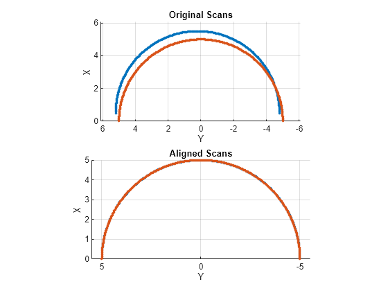
Use the transformScan function to align the scans by transforming the second scan into the frame of the first scan using the relative pose difference. Plot both the original scans and the aligned scans.

currScan2 = transformScan(currScan,pose);

subplot(2,1,1);
hold on
plot(currScan)
plot(refScan)
title('Original Scans')
hold off

subplot(2,1,2);
hold on
plot(currScan2)
plot(refScan)
title('Aligned Scans')
xlim([0 5])
hold off

Figure contains 2 axes objects. Axes object 1 with title Original Scans, xlabel X, ylabel Y contains 2 objects of type line. One or more of the lines displays its values using only markers Axes object 2 with title Aligned Scans, xlabel X, ylabel Y contains 2 objects of type line. One or more of the lines displays its values using only markers

This example uses the 'fminunc' solver algorithm to perform scan matching. This solver algorithm requires an Optimization Toolbox™ license.

Specify a reference laser scan as ranges and angles.

refRanges = 5*ones(1,300);
refAngles = linspace(-pi/2,pi/2,300);

Using the transformScan (Robotics System Toolbox) function, generate a second laser scan at an x,y offset of (0.5,0.2).

[currRanges,currAngles] = transformScan(refRanges,refAngles,[0.5 0.2 0]);

Match the reference scan and the second scan to estimate the pose difference between them.

pose = matchScans(currRanges,currAngles,refRanges,refAngles,'SolverAlgorithm','fminunc');

Improve the estimate by giving an initial pose estimate.

pose = matchScans(currRanges,currAngles,refRanges,refAngles,...
                  'SolverAlgorithm','fminunc','InitialPose',[-0.4 -0.1 0]);

Use the transformScan function to align the scans by transforming the second scan into the frame of the first scan using the relative pose difference. Plot both the original scans and the aligned scans.

[currRanges2,currAngles2] = transformScan(currRanges,currAngles,pose);

[x1, y1] = pol2cart(refAngles,refRanges);
[x2, y2] = pol2cart(currAngles,currRanges);
[x3, y3] = pol2cart(currAngles2,currRanges2);

subplot(1,2,1)
plot(x1,y1,'o',x2,y2,'*r')
title('Original Scans')
subplot(1,2,2)
plot(x1,y1,'o',x3,y3,'*r')
title('Aligned Scans')

Figure contains 2 axes objects. Axes object 1 with title Original Scans contains 2 objects of type line. One or more of the lines displays its values using only markers Axes object 2 with title Aligned Scans contains 2 objects of type line. One or more of the lines displays its values using only markers

Input Arguments

collapse all

Current lidar scan readings, specified as a lidarScan object.

Your lidar scan can contain Inf and NaN values, but the algorithm ignores them.

Reference lidar scan readings, specified as a lidarScan object.

Your lidar scan can contain Inf and NaN values, but the algorithm ignores them.

Current laser scan ranges, specified as a vector. Ranges are given as distances to objects measured from the laser sensor.

Your laser scan ranges can contain Inf and NaN values, but the algorithm ignores them.

Current laser scan angles, specified as a vector in radians. Angles are given as the orientations of the corresponding range measurements.

Reference laser scan ranges, specified as a vector in meters. Ranges are given as distances to objects measured from the laser sensor.

Your laser scan ranges can contain Inf and NaN values, but the algorithm ignores them.

Reference laser scan angles, specified as a vector in radians. Angles are given as the orientations of the corresponding range measurements.

Name-Value Arguments

Specify optional pairs of arguments as Name1=Value1,...,NameN=ValueN, where Name is the argument name and Value is the corresponding value. Name-value arguments must appear after other arguments, but the order of the pairs does not matter.

Before R2021a, use commas to separate each name and value, and enclose Name in quotes.

Example: "InitialPose",[1 1 pi/2]

Optimization algorithm, specified as either "trust-region" or "fminunc". Using "fminunc" requires an Optimization Toolbox™ license.

Initial guess of the current pose relative to the reference laser scan, specified as the comma-separated pair consisting of "InitialPose" and an [x y theta] vector. [x y] is the translation in meters and theta is the rotation in radians.

Length of a cell side in meters, specified as the comma-separated pair consisting of "CellSize" and a numeric scalar. matchScans uses the cell size to discretize the space for the NDT algorithm.

Tuning the cell size is important for proper use of the NDT algorithm. The optimal cell size depends on the input scans and the environment of your robot. Larger cell sizes can lead to less accurate matching with poorly sampled areas. Smaller cell sizes require more memory and less variation between subsequent scans. Sensor noise influences the algorithm with smaller cell sizes as well. Choosing a proper cell size depends on the scale of your environment and the input data.

Maximum number of iterations, specified as the comma-separated pair consisting of "MaxIterations" and a scalar integer. A larger number of iterations results in more accurate pose estimates, but at the expense of longer execution time.

Lower bound on the change in NDT score, specified as the comma-separated pair consisting of "ScoreTolerance" and a numeric scalar. The NDT score is stored in the Score field of the output stats structure. Between iterations, if the score changes by less than this tolerance, the algorithm converges to a solution. A smaller tolerance results in more accurate pose estimates, but requires a longer execution time.

Output Arguments

collapse all

Pose of current scan relative to the reference scan, returned as [x y theta], where [x y] is the translation in meters and theta is the rotation in radians.

Scan matching statistics, returned as a structure with the following fields:

  • Score — Numeric scalar representing the NDT score while performing scan matching. This score is an estimate of the likelihood that the transformed current scan matches the reference scan. Score is always nonnegative. Larger scores indicate a better match.

  • Hessian — 3-by-3 matrix representing the Hessian of the NDT cost function at the given pose solution. The Hessian is used as an indicator of the uncertainty associated with the pose estimate.

References

[1] Biber, P., and W. Strasser. "The Normal Distributions Transform: A New Approach to Laser Scan Matching." Intelligent Robots and Systems Proceedings. 2003.

[2] Magnusson, Martin. "The Three-Dimensional Normal-Distributions Transform -- an Efficient Representation for Registration, Surface Analysis, and Loop Detection." PhD Dissertation. Örebro University, School of Science and Technology, 2009.

Extended Capabilities

Version History

Introduced in R2019b