Lineare Regression mit einer Prädiktorvariable

Live Script öffnen

Eine einfache lineare Regression beschreibt die Beziehung zwischen einer einzelnen Prädiktorvariable und einer Reaktionsvariable. Ein lineares Regressionsmodell ist nützlich, um zu verstehen, wie Änderungen des Prädiktors sich auf die Reaktion auswirken.

Dieses Beispiel demonstriert die Anpassung, Visualisierung und Validierung einfacher linearer Regressionsmodelle verschiedener Grade mithilfe der Funktionen polyfit und polyval. Informationen zur Anpassung und Visualisierung eines Modells mit dem Basic Fitting Tool finden Sie unter Interactively Fit Data and Visualize Model.

Verwenden Sie eine einfache lineare Regression, wenn:

Sie eine Prädiktorvariable haben.
Die Beziehung zwischen Prädiktor und Reaktion in den Koeffizienten linear ist.
Sie die Auswirkung des Prädiktors auf die Reaktion quantifizieren möchten.

Plotten von Daten

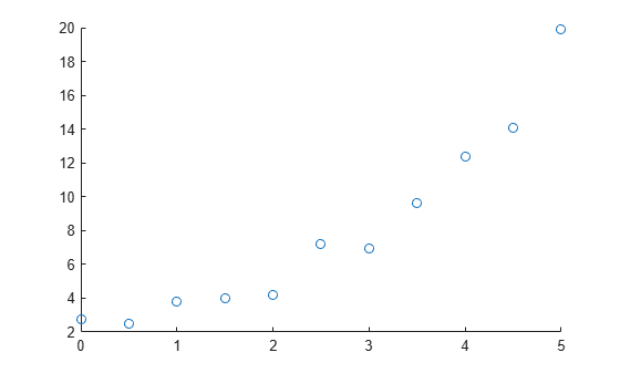
Beginnen Sie, indem Sie Ihre Daten plotten, um mögliche Grade für Ihre Polynomanpassung zu ermitteln.

Erstellen und visualisieren Sie beispielsweise eine Beispiel-Prädiktorvariable x und eine Beispiel-Reaktionsvariable y. Diese Visualisierung deutet darauf hin, dass eine lineare oder quadratische Anpassung die Beziehung zwischen Prädikator- und Reaktionsvariable gut beschreiben könnte.

x = [0:0.5:5]';
y = [2.73 2.50 3.79 3.98 4.21 7.18 6.95 9.63 12.39 14.10 19.93]';
scatter(x,y)

Figure contains an axes object. The axes object contains an object of type scatter.

Anpassen eines Modells ersten Grades

Passen Sie ein (lineares) Modell ersten Grades an die Daten an, indem Sie die Funktion polyfit verwenden. Geben Sie zwei Ausgabeargumente an, um die polynomialen Koeffizienten sowie die Fehlerschätzstruktur zurückzugeben.

[pLinear,SLinear] = polyfit(x,y,1)

pLinear = 1×2

    3.1316    0.1155

SLinear = struct with fields:
           R: [2×2 double]
          df: 9
       normr: 6.3071
    rsquared: 0.8715

Zeigen Sie das angepasste Modell an.

eqLinear = "Linear: " + pLinear(1) + "x + " + pLinear(2)

eqLinear = 
"Linear: 3.1316x + 0.11545"

Anpassen eines höhergradigen Modells

Wenn ein Modell ersten Grades die Beziehung zwischen der Prädiktor- und der Reaktionsvariable nicht angemessen beschreiben kann, können Sie ein höhergradiges Modell anpassen. Passen Sie beispielsweise ein (quadratisches) Modell zweiten Grades an die Daten an, indem Sie die Funktion polyfit verwenden. Geben Sie zwei Ausgabeargumente an, um die polynomialen Koeffizienten sowie die Fehlerschätzstruktur zurückzugeben.

[pQuad,SQuad] = polyfit(x,y,2)

pQuad = 1×3

    0.7898   -0.8175    3.0773

SQuad = struct with fields:
           R: [3×3 double]
          df: 8
       normr: 2.5152
    rsquared: 0.9796

Zeigen Sie das angepasste Modell an.

eqQuad = "Quadratic: " + pQuad(1) + "x^2 + " + pQuad(2) + "x + " + pQuad(3)

eqQuad = 
"Quadratic: 0.78984x^2 + -0.81755x + 3.0773"

Vergleichen von Modellen

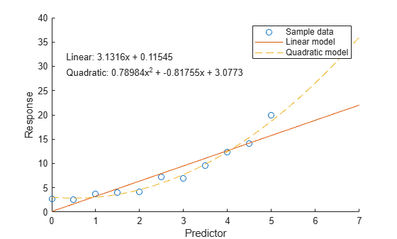
Um Modelle mithilfe eines Diagramms zu vergleichen, werten Sie zunächst jedes Modell bei den Abfragepunkten aus und geben Sie die prognostizierten Reaktionswerte mithilfe der Funktion polyval zurück. Visualisieren Sie daraufhin die Daten und beide Modelle.

Berechnen Sie beispielsweise die Reaktionswerte für das lineare Modell und das quadratische Modell über einen feineren Bereich von x-Werten.

xQuery = [0:0.05:7]';
yLinear = polyval(pLinear,xQuery);
yQuad = polyval(pQuad,xQuery);

Wenn das höhergradige Modell die Reaktionswerte nicht gut prognostizieren kann, könnte dies auf eine Überanpassung hinweisen. Informationen zur Validierung Ihres Modells und zur Auswahl der angemessenen Modellkomplexität finden Sie im Abschnitt Validieren von Modellen.

Plotten Sie daraufhin die Stichprobendaten und die Modelldaten.

scatter(x,y)
hold on
plot(xQuery,yLinear,"-")
plot(xQuery,yQuad,"--")
hold off

xlabel("Predictor")
ylabel("Response")
legend(["Sample data" "Linear model" "Quadratic model"])
text(0.3,30,[eqLinear eqQuad])

Figure contains an axes object. The axes object with xlabel Predictor, ylabel Response contains 4 objects of type scatter, line, text. These objects represent Sample data, Linear model, Quadratic model.

Validieren von Modellen

Um ein Modell zu validieren, berechnen Sie den Bestimmtheitskoeffizienten (R-Quadrat) oder den angepassten Bestimmtheitskoeffizienten (angepasstes R-Quadrat). Ein Wert, der nahe an 1 liegt, weist auf eine gute Anpassung hin.

Validieren eines linearen Modells mit R-Quadrat

Bei einem Modell ersten Grades können Sie mithilfe der von der polyfit-Funktion zurückgegebenen Fehlerschätzstruktur auf den R-Quadrat-Wert zugreifen. Fragen Sie beispielsweise das Feld rsquared in SLinear ab.

linearR2 = SLinear.rsquared

linearR2 = 
0.8715

Validieren höhergradiger Modelle mit angepasstem R-Quadrat

Bei höhergradigen Modellen mit mehr Elementen steigt der R-Quadrat-Wert üblicherweise an und weist auf eine engere Anpassung an die Beobachtungsdaten hin. Diese Modelle unterliegen jedoch einem höheren Risiko einer Überanpassung.

Überanpassung tritt auf, wenn ein Modell die Ursprungsdaten (einschließlich Rauschen) zu eng beschreibt und kein guter Prädiktor mit neuen Daten ist.

Um die Prognosequalität und Modellkomplexität zu balancieren, können Sie das Modell mithilfe des angepassten R-Quadrat-Werts validieren, der einen Punktabzug für die Anzahl Prädiktoren umfasst. Sie berechnen den angepassten R-Quadrat-Wert mithilfe dieser Gleichung, wobei $R^{2}$ für den Wert des Felds rsquared in der Fehlerschätzstruktur steht, $N$ für die Anzahl Beobachtungen in Ihren Daten steht und $d$ für den Grad Ihres Modells steht.

$R_{a d j u s t e d}^{2} = 1 - \frac{(1 - R^{2}) (N - 1)}{N - d - 1}$

Berechnen Sie beispielsweise den angepassten R-Quadrat-Wert des quadratischen Modells.

quadAdjRsq = 1 - (1 - SQuad.rsquared) * (numel(y) - 1) / (numel(y) - 2 - 1)

quadAdjRsq = 
0.9744

Berechnen des maximalen Prognosefehlers jedes Modells

Zudem können Sie ein Modell validieren, indem Sie den größten Fehler zwischen den Modellprognosen und den Stichprobendaten berechnen. Ein kleiner Maximalfehler relativ zu den Datenwerten weist auf eine gute Anpassung hin.

Berechnen Sie beispielsweise den Maximalfehler des linearen Modells und des quadratischen Modells.

Lia = ismember(xQuery,x);
linearMaxError = max(abs(yLinear(Lia) - y))

linearMaxError = 
4.1564

quadMaxError = max(abs(yQuad(Lia) - y))

quadMaxError = 
1.2926

Siehe auch

Funktionen

polyfit | polyval

Themen

Interactively Fit Data and Visualize Model
Linear Regression with Nonpolynomial Terms
Linear Regression with Multiple Predictor Variables
Erstellen und Auswerten von Polynomen
Linear Regression Workflow (Statistics and Machine Learning Toolbox)
Fit Polynomial Models (Curve Fitting Toolbox)