dsphdl.IFFT
Compute inverse fast Fourier transform (IFFT)
Description
The dsphdl.IFFT
System object™ provides two architectures that implement the algorithm for FPGA and ASIC
applications. You can select an architecture that optimizes for either throughput or area.
'Streaming Radix 2^2'— Use this architecture for high-throughput applications. This architecture supports scalar or vector input data. You can achieve gigasamples-per-second (GSPS) throughput, also called super sample rates, using vector input. Since 2025a, this architecture also supports specifying the FFT size by using an input port, when you use scalar input data.'Burst Radix 2'— Use this architecture for a minimum resource implementation, especially with large fast-Fourier-transform (FFT) sizes. Your system must be able to tolerate bursty data and higher latency. This architecture supports only scalar input data.
The object accepts real or complex data, provides hardware-friendly control signals, and has optional output frame control signals.
To calculate the inverse fast Fourier transform:
Create the
dsphdl.IFFTobject and set its properties.Call the object with arguments, as if it were a function.
To learn more about how System objects work, see What Are System Objects?
Note
You can also generate HDL code for this hardware-optimized algorithm, without creating a MATLAB® script, by using the DSP HDL IP Designer app. The app provides the same interface and configuration options as the System object.
Creation
Description
IFFT_N = dsphdl.IFFTIFFT_N, that performs a fast Fourier transform.
IFFT_N = dsphdl.IFFT(Name=Value)
Example: ifft128 = dsphdl.IFFT(FFTLength=128)
Properties
Usage
Syntax
Description
[ returns the next
element of the IFFT using the burst Radix 2 architecture. The Y,validOut,ready]
= IFFT_N(X,validIn)ready
signal indicates when the object has memory available to accept new input data. When you
use the burst architecture, you must respect the ready backpressure
signal. For more information, see the Control Signals
section.
To use this syntax, set the Architecture property to 'Burst Radix 2'. For example:
IFFT_N = dsphdl.IFFT(___,Architecture='Burst Radix 2'); ... [y,validOut,ready] = IFFT_N(x,validIn)
[
returns the next element of the IFFT of the size specified. Specify the
Y,validOut,ready]
= IFFT_var(X,validIn,log2FFTLen,loadFFTLen)log2FFTLen input argument as
log2(FFTLength). Set the
loadFFTLen input argument to 1
(true) to capture the value from the input
log2FFTLen argument.
Variable-size FFT designs must respect the ready backpressure
signal. For more information, see the Control Signals
section.
To use this syntax, set the FFTLengthSource property to
'Input port'. For example:
IFFT_var = dsphdl.IFFT(___,Architecture='Streaming Radix 2^2', ...
                       FFTLengthSource='Input port', ...
                       FFTLengthMax=512);
...
[y,validOut,ready] = IFFT_var(x,validIn,log2FFTLen,1)
[y,validOut,ready] = IFFT_var(x,validIn,log2FFTLen,0)
[
also returns frame control signals Y,startOut,endOut,validOut]
= IFFT_N(X,validIn)startOut and
endOut. startOut is 1 (true) with
the first sample of a frame of output data. endOut is
1 (true) with the last sample of a frame of output data.
To use this syntax, set the StartOutputPort and EndOutputPort properties to true. For example:
IFFT_N = dsphdl.IFFT(___,StartOutputPort=true,EndOutputPort=true);
...
[y,startOut,endOut,validOut] = IFFT_N(x,validIn)
[
returns the IFFT, Y,validOut]
= IFFT_N(X,validIn,resetIn)Y, when validIn is
1 (true) and resetIn is 0
(false).
When resetIn is 1 (true), the object stops the current
calculation and clears all internal state.
To use this syntax, set the ResetInputPort property to true. For example:
IFFT_N = dsphdl.IFFT(___,ResetInputPort=true);
...
[y,validOut] = IFFT_N(x,validIn,resetIn)Input Arguments
Output Arguments
Object Functions
To use an object function, specify the
System object as the first input argument. For
example, to release system resources of a System object named obj, use
this syntax:
release(obj)
Examples
Create the specifications and input signal. This example uses a 128-point FFT.
N = 128;
Fs = 40;
t = (0:N-1)'/Fs;
x = sin(2*pi*15*t) + 0.75*cos(2*pi*10*t);
y = x + .25*randn(size(x));
y_fixed = fi(y,1,32,16);
noOp = zeros(1,'like',y_fixed);
Compute the FFT of the signal to use as the input to the IFFT object.
hdlfft = dsphdl.FFT(FFTLength=N,BitReversedOutput=false);
Yf = zeros(1,4*N);
validOut = false(1,4*N);
for loop = 1:1:N
   	  [Yf(loop),validOut(loop)] = hdlfft(complex(y_fixed(loop)),true);
end
for loop = N+1:1:4*N
	  [Yf(loop),validOut(loop)] = hdlfft(complex(noOp),false);
end
Yf = Yf(validOut == 1);
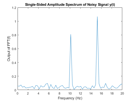
Plot the single-sided amplitude spectrum.
plot(Fs/2*linspace(0,1,N/2),2*abs(Yf(1:N/2)/N))
title('Single-Sided Amplitude Spectrum of Noisy Signal y(t)')
xlabel('Frequency (Hz)')
ylabel('Output of FFT (f)')

Select frequencies that hold the majority of the energy in the signal. The cumsum function does not accept fixed-point arguments, so convert the data back to double.
[Ysort,i] = sort(abs(double(transpose(Yf(1:N)))),1,'descend');
Ysort_d = double(Ysort);
CumEnergy = sqrt(cumsum(Ysort_d.^2))/norm(Ysort_d);
j = find(CumEnergy > 0.9, 1);
     disp(['Number of FFT coefficients that represent 90% of the ', ...
     'total energy in the sequence: ', num2str(j)])
Yin = zeros(N,1);
Yin(i(1:j)) = Yf(i(1:j));
Number of FFT coefficients that represent 90% of the total energy in the sequence: 4
Write a function that creates and calls the IFFT System object™. You can generate HDL from this function.
function [yOut,validOut] = HDLIFFT128(yIn,validIn)
%HDLIFFT128
% Processes one sample of data using the dsphdl.IFFT System object(TM)
% yIn is a fixed-point scalar or column vector.
% validIn is a logical scalar.
% You can generate HDL code from this function.

  persistent ifft128;
  if isempty(ifft128)
    ifft128 = dsphdl.IFFT(FFTLength=128);
  end
  [yOut,validOut] = ifft128(yIn,validIn);
end

% Copyright 2012-2023 The MathWorks, Inc.
Compute the IFFT by calling the function for each data sample.
Xt = zeros(1,3*N);
validOut = false(1,3*N);
for loop = 1:1:N
    [Xt(loop),validOut(loop)] = HDLIFFT128(complex(Yin(loop)),true);
end
for loop = N+1:1:3*N
    [Xt(loop),validOut(loop)] = HDLIFFT128(complex(0),false);
end
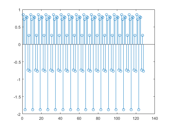
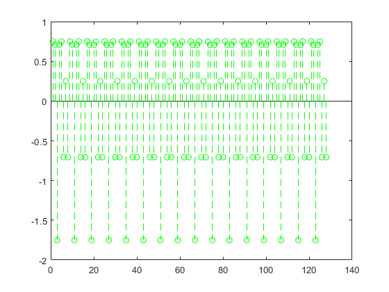
Discard invalid output samples. Then inspect the output and compare it with the input signal. The original input is in green.
Xt = Xt(validOut==1);
Xt = bitrevorder(Xt);
norm(x-transpose(Xt(1:N)))
figure
stem(real(Xt))
figure
stem(real(x),'--g')
ans =

    0.7863


Create the specifications and input signal. This example uses a 128-point FFT and computes the transform over 16 samples at a time.
N = 128;
V = 16;
Fs = 40;
t = (0:N-1)'/Fs;
x = sin(2*pi*15*t) + 0.75*cos(2*pi*10*t);
y = x + .25*randn(size(x));
y_fixed = fi(y,1,32,24);
y_vect = reshape(y_fixed,V,N/V);
Compute the FFT of the signal, to use as the input to the IFFT object.
hdlfft = dsphdl.FFT('FFTLength',N);
loopCount = getLatency(hdlfft,N,V)+N/V;
Yf = zeros(V,loopCount);
validOut = false(V,loopCount);
for loop = 1:1:loopCount
    if ( mod(loop,N/V) == 0 )
        i = N/V;
    else
        i = mod(loop,N/V);
    end
 	  [Yf(:,loop),validOut(loop)] = hdlfft(complex(y_vect(:,i)),(loop<=N/V));
end
Plot the single-sided amplitude spectrum.
C = Yf(:,validOut==1);
Yf_flat = C(:);
Yr = bitrevorder(Yf_flat);
plot(Fs/2*linspace(0,1,N/2),2*abs(Yr(1:N/2)/N))
title('Single-Sided Amplitude Spectrum of Noisy Signal y(t)')
xlabel('Frequency (Hz)')
ylabel('Output of FFT(f)')
Select frequencies that hold the majority of the energy in the signal. The cumsum function doesn't accept fixed-point arguments, so convert the data back to double.
[Ysort,i] = sort(abs(double(Yr(1:N))),1,'descend');
CumEnergy = sqrt(cumsum(Ysort.^2))/norm(Ysort);
j = find(CumEnergy > 0.9, 1);
     disp(['Number of FFT coefficients that represent 90% of the ', ...
     'total energy in the sequence: ', num2str(j)])
Yin = zeros(N,1);
Yin(i(1:j)) = Yr(i(1:j));
YinVect = reshape(Yin,V,N/V);
Number of FFT coefficients that represent 90% of the total energy in the sequence: 4
Write a function that creates and calls the IFFT System object™. You can generate HDL from this function.
function [yOut,validOut] = HDLIFFT128V16(yIn,validIn)
%HDLFFT128V16
% Processes 16-sample vectors of FFT data
% yIn is a fixed-point column vector.
% validIn is a logical scalar value.
% You can generate HDL code from this function.

  persistent ifft128v16;
  if isempty(ifft128v16)
    ifft128v16 = dsphdl.IFFT(FFTLength=128)
  end
  [yOut,validOut] = ifft128v16(yIn,validIn);
end

% Copyright 2012-2023 The MathWorks, Inc.
Compute the IFFT by calling the function for each data sample.
Xt = zeros(V,loopCount);
validOut = false(V,loopCount);
for loop = 1:1:loopCount
    if ( mod(loop,N/V) == 0 )
        i = N/V;
    else
        i = mod(loop,N/V);
    end
 	  [Xt(:,loop),validOut(loop)] = HDLIFFT128V16(complex(YinVect(:,i)),(loop<=N/V));
end
ifft128v16 =

  dsphdl.IFFT with properties:

   Main
             Architecture: 'Streaming Radix 2^2'
          FFTLengthSource: 'Property'
                FFTLength: 128
    ComplexMultiplication: 'Use 4 multipliers and 2 adders'
        BitReversedOutput: true
         BitReversedInput: false
                Normalize: true

  Use get to show all properties
Discard invalid output samples. Then inspect the output and compare it with the input signal. The original input is in green.
C = Xt(:,validOut==1);
Xt = C(:);
Xt = bitrevorder(Xt);
norm(x-Xt(1:N))
figure
stem(real(Xt))
figure
stem(real(x),'--g')
ans =

    0.7863
The latency of the object varies with the FFT length and the vector size. Use the getLatency function to find the latency of a particular configuration. The latency is the number of cycles between the first valid input and the first valid output, assuming that the input is contiguous.
Create a new dsphdl.IFFT object and request the latency.
hdlifft = dsphdl.IFFT(FFTLength=512);
L512 = getLatency(hdlifft)
L512 =
599
Request hypothetical latency information about a similar object with a different FFT length. The properties of the original object do not change. When you do not specify a vector length, the function assumes scalar input data.
L256 = getLatency(hdlifft,256)
L256 =
329
N = hdlifft.FFTLength
N =
512
Request hypothetical latency information of a similar object that accepts eight-sample vector input.
L256v8 = getLatency(hdlifft,256,8)
L256v8 =
93
Enable scaling at each stage of the IFFT. The latency does not change.
hdlifft.Normalize = true;
L512n = getLatency(hdlifft)
L512n =
599
Request the same output order as the input order. This setting increases the latency because the object must collect the output before reordering.
hdlifft.BitReversedOutput = false;
L512r = getLatency(hdlifft)
L512r =
1078
Algorithms
The streaming Radix 2^2 architecture implements a low-latency architecture. It saves resources compared to a streaming Radix 2 implementation by factoring and grouping the FFT equation. The architecture has log4(N) stages. Each stage contains two single-path delay feedback (SDF) butterflies with memory controllers. When you use vector input, each stage operates on fewer input samples, so some stages reduce to a simple butterfly, without SDF.
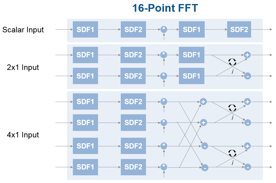
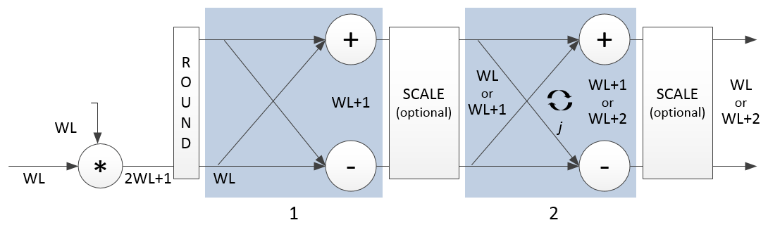
The first SDF stage is a regular butterfly. The second stage multiplies the outputs of the first stage by –j. To avoid a hardware multiplier, the block swaps the real and imaginary parts of the inputs, and again swaps the imaginary parts of the resulting outputs. Each stage rounds the result of the twiddle factor multiplication to the input word length. The twiddle factors have two integer bits, and the rest of the bits are used for fractional bits. The twiddle factors have the same bit width as the input data, WL. The twiddle factors have two integer bits, and WL-2 fractional bits.
If you enable scaling, the algorithm divides the result of each butterfly stage by 2. Scaling at each stage avoids overflow, keeps the word length the same as the input, and results in an overall scale factor of 1/N. If scaling is disabled, the algorithm avoids overflow by increasing the word length by 1 bit at each stage. The diagram shows the butterflies and internal word lengths of each stage, not including the memory.
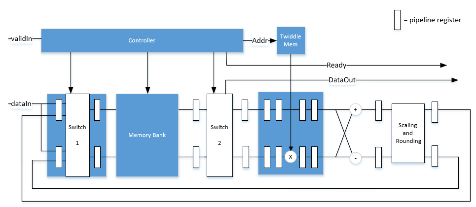
The burst Radix 2 architecture implements the FFT by using a single complex butterfly multiplier. The algorithm cannot start until it has stored the entire input frame, and it cannot accept the next frame until computations are complete. The output ready port indicates when the algorithm is ready for new data. The diagram shows the burst architecture, with pipeline registers.
When you use this architecture, your input data must comply with the ready backpressure signal.
The algorithm processes input data only when the input valid port is 1. Output data is valid only when the output valid port is 1.
When the optional input reset port is 1, the algorithm stops the current calculation and clears all internal states. The algorithm begins new calculations when reset port is 0 and the input valid port starts a new frame.
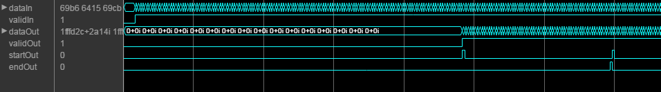
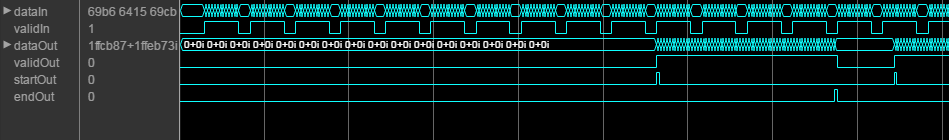
This diagram shows the input and output valid input values for contiguous scalar input data, streaming Radix 2^2 architecture, an FFT length of 1024, and a vector size of 16.
The diagram also shows the optional start and end outputs that indicate frame boundaries. If you enable the start output, the start output pulses for one cycle with the first valid output of the frame. If you enable the end output, the end output pulses for one cycle with the last valid output of the frame.
If you apply continuous input frames, the output will also be continuous after the initial latency.
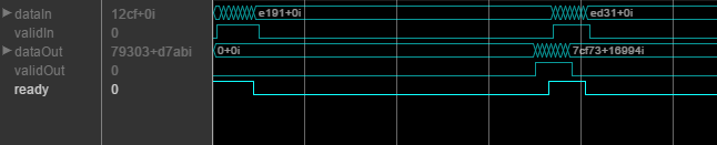
The valid input can be noncontiguous. The algorithm processes data accompanied by a validsignal as it arrives, and stores the resulting data until a frame is filled. Then the algorithm returns contiguous output samples in a frame of N (FFT length) cycles. This diagram shows noncontiguous input and contiguous output for an FFT length of 512 and a vector size of 16.
When you use the burst architecture, you cannot provide the next frame of input data until
memory space is available. The ready output indicates when the
algorithm can accept new input data. The algorithm sets the ready
output to 1 (true) when it can accept data, and to
0 (false) when it is processing and cannot accept
more data. If the upstream part of your design has continuous input data and synchronously
reacts to ready before halting input, then one extra cycle of input
data can arrive at the port. This data is the beginning of the next frame. To support
synchronous control logic, the block reserves room to store this extra data while processing
the current frame. For more detail about this extra data, see the annotated waveform in the
Latency
section.
Variable-size FFT designs must also respect the ready signal. When
you load a new FFT length, the algorithm sets ready to
0 (false) while it updates internal logic with the
new size. If the algorithm is processing a previous frame when you load a new FFT size, the
algorithm finishes the frame and then updates internal logic to use the new size.
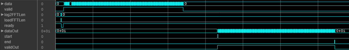
The first waveform shows loading the input size before any frame is processed. The
algorithm sets the ready signal to 0
(false) for 4 cycles while it updates internal logic with the new
size, and then sets ready to 1
(true) again. The waveform shows new input data and
valid set to 1 (true) once
the ready signal is 1 (true)
again.
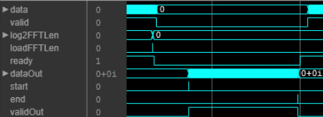
The next waveform shows loading a new FFT size while a frame is processing. When you load
a new size, the algorithm sets the ready signal to 0
(false). You can continue to provide the rest of the current input
frame. The block sets ready to 1
(true) when it has completed the current frame and updated the
internal logic with the new size. You can apply the next frame, of the new size, once the
ready signal is 1 (true).
The latency varies with the FFT length and the vector size. Use the getLatency
function to find the latency of a particular configuration. The latency is the number of
cycles between the first valid input and the first valid output, assuming that the input is
contiguous.
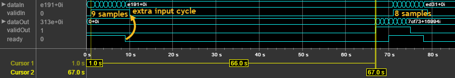
When using the burst
architecture, if the upstream part of your design has continuous input data and synchronously
reacts to ready before halting input, then one extra cycle of input data
can arrive at the port. This data is the beginning of the next frame. To support synchronous
control logic, the block reserves room to store this extra data while processing the current
frame. Due to this one cycle advance, the observed latency of the later frames (cycles from
first input valid to first output valid) is one cycle
shorter than the reported latency. The number of cycles between when ready
port is 0 (false) and the output
valid port is 1 (true) is always
latency – FFTLength.