Discrete-Time Signals

Time and Frequency Terminology

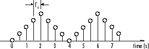
Simulink^® models can process both discrete-time and continuous-time signals. Models built with the DSP System Toolbox™ are intended to process discrete-time signals only. A discrete-time signal is a sequence of values that correspond to particular instants in time. The time instants at which the signal is defined are the signal's sample times, and the associated signal values are the signal's samples. Traditionally, a discrete-time signal is considered to be undefined at points in time between the sample times. For a periodically sampled signal, the equal interval between any pairs of consecutive sample times is the signal's sample period T_s. The sample rate F_s is the reciprocal of the sample period, or 1/T_s. The sample rate is the number of samples in the signal per second.

This 7.5-second triangle wave segment has a sample period of 0.5 seconds, and sample times of 0.0, 0.5, 1.0, 1.5, ...,7.5. The sample rate of the sequence is therefore 1/0.5, or 2 Hz.

A number of different terms are used to describe the characteristics of discrete-time signals found in Simulink models. This table lists terms that are frequently used to describe how various blocks operate on sample-based and frame-based signals.

Term	Symbol	Units	Notes
Sample period	T_sT_siT_so	Seconds	The time interval between consecutive samples in a sequence, as the input to a block (T_si) or the output from a block (T_so).
Frame period	T_fT_fiT_fo	Seconds	The time interval between consecutive frames in a sequence, as the input to a block (T_fi) or the output from a block (T_fo).
Signal period	T	Seconds	The time elapsed during a single repetition of a periodic signal.
Sample frequency	F_s	Hz (samples per second)	The number of samples per unit time, F_{s =}1/T_s.
Frequency	f	Hz (cycles per second)	The number of repetitions per unit time of a periodic signal or signal component, f = 1/T.
Nyquist rate		Hz (cycles per second)	The minimum sample rate that avoids aliasing, usually twice the highest frequency in the signal being sampled.
Nyquist frequency	f_nyq	Hz (cycles per second)	Twice the highest frequency present in the signal.
Normalized frequency	f_n	Two cycles per sample	Frequency (linear) of a periodic signal normalized to half the sample rate, f_n = ω/π = 2f/F_s.
Angular frequency	Ω	Radians per second	Frequency of a periodic signal in angular units, Ω = 2πf.
Digital (normalized angular) frequency	ω	Radians per sample	Frequency (angular) of a periodic signal normalized to the sample rate, ω = Ω/F_s = πf_n.

Note

In the block dialogs, the term sample time is used to refer to the sample period T_s. For example, the Sample time parameter in the Signal From Workspace block specifies the imported signal's sample period.

Recommended Settings for Discrete-Time Simulations

Simulink allows you to select from several different simulation solver algorithms. You can access these solver algorithms from a Simulink model:

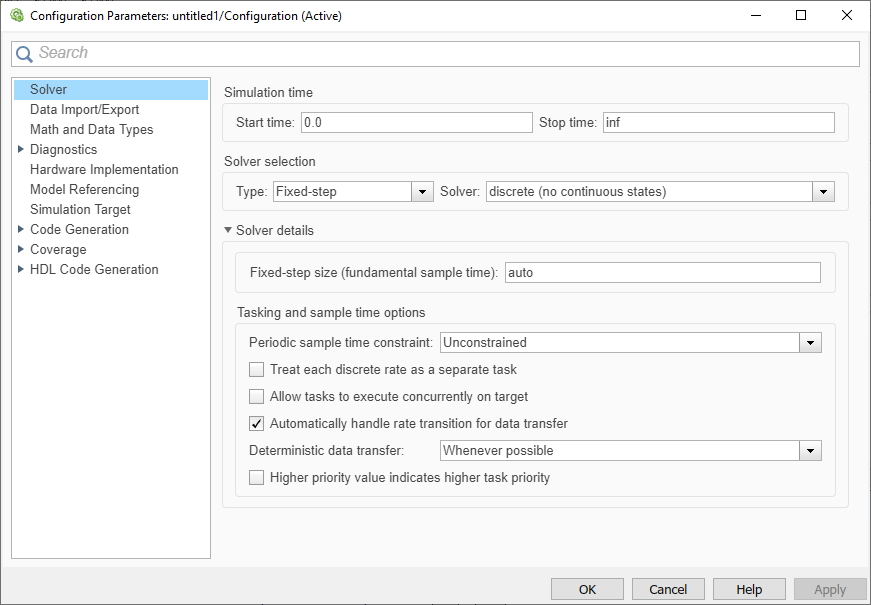
On the Modeling tab, click Model Settings. The Configuration Parameters dialog box opens.
The selections you make in the Solver pane determine how discrete-time signals are processed in Simulink. The recommended Solver settings for signal processing simulations are:
- Type: Fixed-step
- Solver: Discrete (no continuous states)
- Fixed-step size (fundamental sample time): auto
- Treat each discrete rate as a separate task: Off

You can automatically set these solver options for all new models by using the DSP Simulink model templates. For more information, see Configure the Simulink Environment for Signal Processing Models.

Simulink Tasking Modes

When the solver type is set to Fixed-step, Simulink operates in two tasking modes:

Single-tasking mode
Multitasking mode

On the Modeling tab, click Model Settings. The Configuration Parameters dialog box opens. In the Solver pane, select Type > Fixed-step. Expand Solver details. To specify the multitasking mode, select Treat each discrete rate as a separate task. To specify the single-tasking mode, clear Treat each discrete rate as a separate task.

If you select the Treat each discrete rate as a separate task parameter, the single-tasking mode is still used in these cases:

If your model contains one sample time
If your model contains a continuous and a discrete sample time, and the fixed-step size is equal to the discrete sample time

For a typical model that operates on a single rate, Simulink selects the single-tasking mode.

Fixed-step single-tasking mode

In the fixed-step, single-tasking mode, discrete-time signals differ from the prototype described in Time and Frequency Terminology by remaining defined between sample times. For example, the representation of the discrete-time triangle wave looks like this.

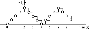
This signal's value at t = 3.112 seconds is the same as the signal's value at t = 3 seconds. In the fixed-step, single-tasking mode, a signal's sample times are the instants where the signal is allowed to change values rather than where the signal is defined. Between sample times, the signal takes on the value at the previous sample time.

As a result, in the fixed-step, single-tasking mode, Simulink permits cross-rate operations such as the addition of two signals of different rates. This is explained further in Cross-Rate Operations.

Other Settings for Discrete-Time Simulations

It is useful to know how the other solver options available in Simulink affect discrete-time signals. In particular, you should be aware of the properties of discrete-time signals under these settings:

Type: Fixed-step, select Treat each discrete rate as a separate task to enable the multitasking mode.
When the fixed-step, multitasking solver is selected, discrete signals in Simulink are undefined between sample times. Simulink generates an error when operations attempt to reference the undefined region of a signal, as, for example, when signals with different sample rates are added.
Type: Variable-step (the Simulink default solver)
When the Variable-step solver is selected, discrete-time signals remain defined between sample times, just as in the fixed-step, single-tasking case described in Recommended Settings for Discrete-Time Simulations. When the Variable-step solver is selected, cross-rate operations are allowed by Simulink.

For a typical model containing multiple rates, Simulink selects the multitasking mode.

Cross-Rate Operations

This example uses:

Open Model

When the fixed-step, multitasking solver is selected, discrete signals in Simulink are undefined between sample times. Therefore, to perform cross-rate operations like the addition of two signals with different sample rates, you must convert the two signals to a common sample rate. Several blocks in the Signal Operations and Multirate Filters libraries can accomplish this task. See Convert Sample and Frame Rates in Simulink Using Rate Conversion Blocks for more information. Rate change can occur implicitly depending on the diagnostic settings. However, this is not recommended. See Multitask data transfer (Simulink), Single task data transfer (Simulink). By requiring explicit rate conversions for cross-rate operations in discrete mode, Simulink helps you identify sample rate conversion issues early in the design process.

When the Variable-step solver or fixed-step, single-tasking solver is selected, discrete-time signals remain defined between sample times. Therefore, if you sample the signal with a rate or phase that is different from the signal's own rate and phase, you will still measure meaningful values:

Open the ex_sum_tut1 model. The Cross-Rate Sum Example model opens. This model adds two signals with different sample periods.

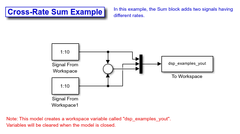
Double-click the upper Signal From Workspace block. The Signal From Workspace dialog box opens.

Set the Sample time parameter to 1. This creates a fast signal (Ts = 1) with sample times 1, 2, 3, ... and so on.

Double-click the lower Signal From Workspace block. Set the Sample time parameter to 2. This creates a slow signal (Ts = 2) with sample times 1, 3, 5, ... and so on.

On the Debug tab, under Information Overlays, select Colors. Selecting Colors allows you to see the different sampling rates in action. For more information about the color coding of the sample times, see View Sample Time Information (Simulink).

Run the model.

Note: Using the DSP Simulink model templates with cross-rate operations generates errors even though a fixed-step, single-tasking solver is selected. This is due to the fact that Single task data transfer is set to error in the Sample Time pane of the Diagnostics section of the Configuration Parameters dialog box.

At the MATLAB command line, type dsp_examples_yout. The following output is displayed.

dsp_examples_yout =

     1     1     2
     2     1     3
     3     2     5
     4     2     6
     5     3     8
     6     3     9
     7     4    11
     8     4    12
     9     5    14
    10     5    15
     0     6     6

The first column of the matrix is the fast signal (Ts = 1). The second column of the matrix is the slow signal (Ts = 2). The third column is the sum of the two signals. As expected, the slow signal changes once every 2 seconds, half as often as the fast signal. Nevertheless, the slow signal is defined at every moment because Simulink holds the previous value of the slower signal during time instances that the block doesn't run.

In general, for Variable-step and the fixed-step single-tasking modes, when you measure the value of a discrete signal between sample times, you are observing the value of the signal at the previous sample time.