Generate RoadRunner Scene Using Labeled Camera Images and Raw Lidar Data

This example shows how to generate a RoadRunner scene containing add or drop lanes with junctions using labeled camera images, raw lidar data, and GPS waypoints.

You can create a virtual scene from recorded sensor data that represents real-world roads and use it to perform safety assessments for automated driving applications.

By combining camera images, lidar point clouds, and GPS waypoints you can accurately reconstruct a road scene that contains lane information and junctions. Camera images enable you to easily identify scene elements, such as lane markings and road boundaries, while lidar point clouds enable you to accurately measure their distances and depth. Additionally, you can improve the labeling of lane boundaries in images by using a variety of lane detectors that perform reliably regardless of the camera used. In contrast, labeling lane boundaries directly in lidar point clouds is difficult, as they generally do not contain RGB information and the accuracy of lane detectors for point clouds is dependent on the sensor used. This example fuses lane boundary labels from images with lidar point clouds to generate an accurate scene.

In this example, you:

• Load a sequence of lidar point clouds, lane boundary-labeled images, and GPS waypoints.

• Divide the scene into segments with a fixed number of lane boundaries in each segment.

• Map the lane boundary labels across the entire sequence.

• Fuse the camera lane boundary labels with the lidar point clouds.

• Extract the lane boundary points from the fused point clouds.

• Generate a RoadRunner HD Map from the extracted lane boundary points.

The workflow in this example requires:

• labeled camera images,

• raw lidar point cloud data,

• GPS waypoints,

• calibration information between the camera and lidar coordinate systems, and

• calibration information between the lidar and world coordinate systems.

Load Sensor Data and Lane Boundary Labels

This example requires the Scenario Builder for Automated Driving Toolbox™ support package. Check if the support package is installed and, if it is not installed, install it using the Get and Manage Add-Ons.

checkIfScenarioBuilderIsInstalled

Download a ZIP file containing a subset of sensor data from the PandaSet data set, and then unzip the file. This file contains data for a continuous sequence of 160 point clouds and images. The data also contains lane boundary labels in the form of pixel coordinates. The data stores these labels as a groundTruthMultisignal object. Alternatively, you can obtain lane boundary labels using a lane boundary detector. For more information, see Extract Lane Information from Recorded Camera Data for Scene Generation.

dataFolder = tempdir;
dataFilename = "PandasetSceneGeneration.zip";
url = "https://ssd.mathworks.com/supportfiles/driving/data/" + dataFilename;
filePath = fullfile(dataFolder,dataFilename);
if ~isfile(filePath)
    websave(filePath,url);
end
unzip(filePath,dataFolder)
dataset = fullfile(dataFolder,"PandasetSceneGeneration");

Load the downloaded data set into the workspace using the helperLoadData function.

[imds,pcds,sensor,gTruth,calibration,gps,timestamps] = helperLoadExampleData(dataset);

The output arguments of the helperLoadData function contains:

• imds — Datastore for images, specified as a imageDatastore object.

• pcds — Datastore for lidar point clouds, specified as a fileDatastore object.

• sensor — Camera parameters, specified as a monoCamera object.

• gTruth — Lane boundary labels in pixel coordinate, specified as a groundTruthMultisignal object.

• calibration — Calibration information among camera, lidar, and world coordinate system, specified as a structure.

• gps — GPS coordinates of the ego vehicle, specified as a structure.

• timestamps — Time of capture, in seconds, for the lidar, camera, and GPS data.

Read the first point cloud, the first image, and its corresponding lane boundary labels.

ptCld = read(pcds);
img = read(imds);
boundaries = gTruth.ROILabelData.Camera{1,:}{1};

Overlay the point cloud and the lane boundary labels onto the image and visualize it.

% Create a lidar to camera rigid transformation rigidtform3d object tform
rot = quat2rotm(calibration.camera_to_lidar.heading(1,:));
tran = calibration.camera_to_lidar.position(1,:);
tform = invert(rigidtform3d(rot,tran));

% Downsample the first point cloud data for better visualization and project it onto image coordinate frame
ptCld = pcdownsample(ptCld,gridAverage=0.5);
imPts = projectLidarPointsOnImage(ptCld,sensor.Intrinsics,tform);

% Overlay the projected point cloud onto the image
figure
imshow(img);
hold on
plot(imPts(:,1),imPts(:,2),"b.")

% Overlay lane boundary labels onto the image
for i = 1:length(boundaries)
    boundary = boundaries(i);
    points = boundary.Position;
    plot(points(:,1),points(:,2),LineWidth=3,Color="r")
end

hold off

Note: You can view the labels for all timestamps using the Ground Truth Labeler app by importing gTruth from the workspace or by calling groundTruthLabeler(gTruth).

Visualize geographic map data with GPS trajectory of ego vehicle by using the helperPlotGPS function. Note that, in the figure the ego vehicle is moving from bottom-right to the top-left on the trajectory.

helperPlotGPS(gps);

Divide Scene into Segments with Fixed Number of Lane Boundaries

Divide the scene into smaller segments, each with a fixed number of lane boundaries by using the helperCreateSegments function. Dividing the scene into segments makes it easier to extract geometry of each lane boundary.

The helperCreateSegments function creates subsequent continuous segments with unique number of lane boundaries based on a specified threshold. In the sequence, when there are unequal lane boundaries, a segment is combined with the one before it if the ego vehicle's segmental travel distance is less than the specified threshold distance. Unit of threshold distance is in meters. The returned segments is an M-by-2 array specifying M number of road segments. For each row, the first and second column specifies the start and end indices of a road segment.

% Convert GPS waypoints to Cartesian coordinates
lat = [gps.lat]';
lon = [gps.long]';
alt = [gps.height]';
geoRef = [lat(1),lon(1),alt(1)];
[x,y,z] = latlon2local(lat,lon,alt,geoRef);
waypoints = [x,y,z];

% Divide the scene into segments
segments = helperCreateSegments(gTruth,waypoints,Threshold=18);

Visualize the obtained five segments by using the helperPlotGPS function.

helperPlotGPS(gps,segments);

Map Lane Boundaries

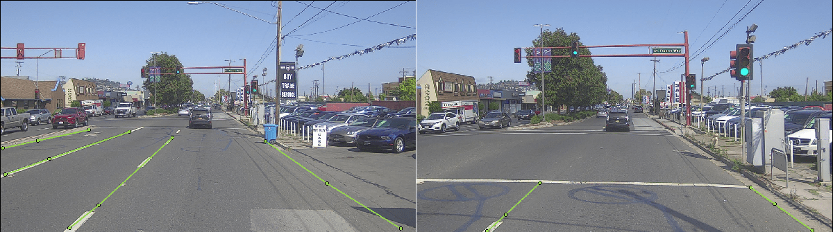
In a road segment, lane boundary labels may be missing for a few frames due to the lane boundary being occluded or moving out of the camera field-of-view. For example, in the image on the right, you can observe that as the ego-vehicle gets closer to the junction, the left-most lane boundaries move outside the camera field-of-view. To extract the points for each lane boundary for the entire sequence, you must map the two visible lane boundaries in the image on the right with the two right-most lane boundaries in the image on the left.

Map the lane boundaries in each frame with the lane boundaries in the previous frame by using the helperMapLaneLabels function. The function returns an M-by-1 cell array, specifying lane boundaries for M segments. For each cell entry, the lane boundaries are sorted in left-to-right order.

mappedBoundaries = cell(size(segments,1),1);
for i = 1:size(segments,1)
    mappedBoundaries{i} = helperMapLaneBoundaryLabels(gTruth,sensor,segments(i,:));
end

Plot the mapped lane boundaries for a frame by using the helperPlotLaneBoundaries function. This function displays the lane boundaries numbered from left to right.

segmentNumber = 2;
frameNumber = 45;
helperPlotLaneBoundaries(imds,mappedBoundaries,segments,segmentNumber,frameNumber);
title("All Lane Boundaries Visible")

Plot the lane boundaries for a subsequent frame. In this figure, you observe that the two right-most lane boundaries are numbered 3 and 4 even after the other boundaries move out of the camera field-of-view.

segmentNumber = 2;
frameNumber = 52;
helperPlotLaneBoundaries(imds,mappedBoundaries,segments,segmentNumber,frameNumber);
title("Only Right Lane Boundaries Visible")

Fuse Lane Boundary Labels with Lidar Point Clouds

Return to the start of the datstores. Overlay the lane boundary labels onto the images and fuse the images with the corresponding point clouds for all timestamps by using the helperFuseCameraToLidar function. The function returns an array of pointCloud objects, which contains the fused point clouds for each timestamp. The function associates each lane boundary point in the fused point cloud with an RGB value of [i 0 255-j] where i is the segment number and j is the index of the lane boundary increasing in the left-to-right order. These RGB values are useful to extract the lane boundary points from the point clouds.

% Reset datastores
reset(imds)
reset(pcds)

% Fuse images and lane boundary labels to lidar for each segment
fusedPointCloudArray = pointCloud.empty(length(pcds.Files),0);
for i = 1:size(segments,1)
    fusedPointClouds = helperFuseCameraToLidar(i,segments,mappedBoundaries,imds,pcds,sensor,calibration);
    fusedPointCloudArray = [fusedPointCloudArray;fusedPointClouds];
end

The point clouds are in the lidar sensor coordinate system. Transform the fused point clouds to the world coordinate system and then concatenate them by using the pccat function. Save the concatenated point cloud as a PCD file to enable you to import it into RoadRunner.

Note: If the calibration information between the world coordinate system and lidar coordinate system is not available, you can stitch the point clouds together by using a point cloud registration algorithm. For more information, see 3-D Point Cloud Registration and Stitching.

% Transform point clouds to world coordinate system and concatenate
fusedPointCloudArray = helperTransformPointClouds(fusedPointCloudArray,calibration.lidar_to_world);

% Concatenate point clouds
fusedPointCloud = pccat(fusedPointCloudArray);

% Save point cloud for entire sequence
pcwrite(fusedPointCloud,"fusedPointCloud.pcd",Encoding="compressed")

Visualize the fused point cloud for the entire sequence by using the pcshow function.

figure
pcshow(fusedPointCloud,ColorSource="Color",ViewPlane="XY");
zoom(5)

Extract Lane Boundary Geometry from Fused Point Cloud

To ensure that only points on the road are extracted from the fused point cloud, use the segmentGroundSMRF (Lidar Toolbox) function which extracts the ground plane from the point cloud.

[~,~,fusedPointCloud] = segmentGroundSMRF(fusedPointCloud,ElevationThreshold=0.1,ElevationScale=0.25,SlopeThreshold=0.05);

Extract the lane boundary points by using their corresponding RGB values from the entire sequence of fused point clouds.

% Get lane boundary points from fused point clouds
laneBoundaryPoints = cell(size(segments,1),1);

figure
% Iterate over segments
for i = 1:size(segments,1)

    labels = mappedBoundaries{i};
    segmentPoints = cell(1,size(labels,2));

    % Extract lane boundary points from point clouds
    for n = 1:size(labels,2)
        idx = all(fusedPointCloud.Color == [i, 0, 255-n], 2);
        points = fusedPointCloud.Location(idx,:);
        plot(points(:,1),points(:,2),"b.")
        hold on
        segmentPoints{n} = [segmentPoints{n}; points(:,1:2)];
    end

    laneBoundaryPoints{i} = segmentPoints;
end

title("Boundary Points Extracted from Fused Point Cloud")
hold off

Use the helperSortPointsInTravelDirection function to sort the extracted lane boundary points along the travel direction. This is necessary to ensure that the geometries of the road segments are connected correctly. The function computes the ego-vehicle travel directions by comparing the start and end the x-coordinate of the ego-vehicle waypoints.

laneBoundaryPoints = helperSortPointsInTravelDirection(laneBoundaryPoints,waypoints,segments);

Create RoadRunner HD Map

Create a RoadRunner HD Map from the extracted lane boundary points by using the roadrunnerLaneInfo function. This function automatically connects the geometry of consecutive road segments. Specify the MinJunctionLength argument as 10 to automatically insert a perpendicular road at the junction.

% Delete the empty segments
empty_idx = cellfun(@(x) isempty(x{1}),laneBoundaryPoints);
laneBoundaryPoints(empty_idx) = [];

% Create a RoadRunner HD Map
rrMap = roadrunnerHDMap;
[laneInfo,geographicBoundary] = roadrunnerLaneInfo(laneBoundaryPoints,SmoothingDegree=2,SmoothingFactor=0.4,MinJunctionLength=10);
rrMap.Lanes = laneInfo.Lanes;
rrMap.LaneBoundaries = laneInfo.LaneBoundaries;
rrMap.GeographicBoundary = geographicBoundary;

Visualize the generated RoadRunner HD Map overlayed on the point cloud of the entire sequence.

ax = plot(rrMap);
pcshow(fusedPointCloud,ViewPlane="XY",Parent=ax)
legend("Lane Boundaries","Lane Centers","Point Cloud")

Write the RoadRunner HD Map to a binary file, which you can import into RoadRunner.

write(rrMap,"rrMap.rrhd")

To open RoadRunner using MATLAB®, specify the path to your RoadRunner project. This code shows the path for a sample project folder location in Windows®.

rrProjectPath = "C:\RR\MyProject";

Specify the path to your local RoadRunner installation folder. This code shows the path for the default installation location in Windows.

rrAppPath = "C:\Program Files\RoadRunner R2023a\bin\win64";

Open RoadRunner using the specified path to your project.

rrApp = roadrunner(rrProjectPath,InstallationFolder=rrAppPath);

Specify the RoadRunner HD Map import options. Set the enableOverlapGroupsOptions to false to ensure that a junction is built at the two intersecting roads.

overlapGroupsOptions = enableOverlapGroupsOptions(IsEnabled=false);
buildOptions = roadrunnerHDMapBuildOptions(EnableOverlapGroupsOptions=overlapGroupsOptions);
importOptions = roadrunnerHDMapImportOptions(BuildOptions=buildOptions);

Import the rrMap.rrhd scene into RoadRunner.

importScene(rrApp,fullfile(pwd,"rrMap.rrhd"),"RoadRunner HD Map",importOptions);

You can import the fused point cloud PCD file into RoadRunner, for visual validation of the generated roads with respect to the imported point clouds, by using the Point Cloud Tool (RoadRunner).

Use Lane Marking Tool to mark lane boundaries in the imported road. This figure shows the built road in RoadRunner that contains a junction with add and drop lanes.

Note: Use of the Scene Builder Tool requires a RoadRunner Scene Builder license.