Train Residual Network for Image Classification
This example shows how to create a deep learning neural network with residual connections and train it on CIFAR-10 data. Residual connections are a popular element in convolutional neural network architectures. Using residual connections improves gradient flow through the network and enables training of deeper networks.
For many applications, using a network that consists of a simple sequence of layers is sufficient. However, some applications require networks with a more complex graph structure in which layers can have inputs from multiple layers and outputs to multiple layers. These types of networks are often called directed acyclic graph (DAG) networks. A residual network (ResNet) is a type of DAG network that has residual (or shortcut) connections that bypass the main network layers. In MATLAB, DAG networks are represented by dlnetwork objects. Residual connections enable the parameter gradients to propagate more easily from the output layer to the earlier layers of the network, which makes it possible to train deeper networks. This increased network depth can result in higher accuracies on more difficult tasks.
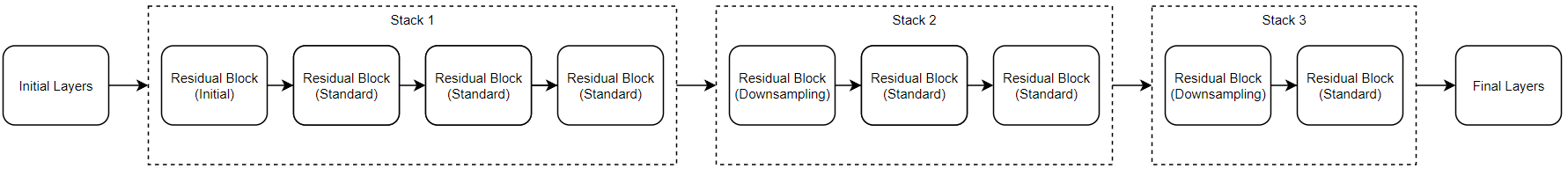
A ResNet architecture is comprised of initial layers, followed by stacks containing residual blocks, and then the final layers. There are three types of residual blocks:
Initial residual block — This block appears at the start of the first stack. This example uses bottleneck components; therefore, this block contains the same layers as the downsampling block, only with a stride of
[1,1]in the first convolutional layer. For more information, seeresnetNetwork.Standard residual block — This block appears in each stack, after the first downsampling residual block. This block appears multiple times in each stack and preserves the activation sizes.
Downsampling residual block — This block appears at the start of each stack (except the first) and only appears once in each stack. The first convolutional unit in the downsampling block downsamples the spatial dimensions by a factor of two.
The depth of each stack can vary, this example trains a residual network with three stacks of decreasing depth. The first stack has depth four, the second stack has depth three, and the final stack has depth two.
Each residual block contains deep learning layers. For more information on the layers in each block, see resnetNetwork.
To create and train a residual network suitable for image classification, follow these steps:
Create a residual network using the
resnetNetworkfunction.Train the network using the
trainnetfunction. The trained network is adlnetworkobject.Perform classification and prediction on new data.
You can also load pretrained residual networks for image classification. For more information, see Pretrained Deep Neural Networks.
Prepare Data
Download the CIFAR-10 data set [1]. The data set contains 60,000 images. Each image is 32-by-32 pixels in size and has three color channels (RGB). The size of the data set is 175 MB. Depending on your internet connection, the download process can take time.
datadir = tempdir;
downloadCIFARData(datadir);
Downloading CIFAR-10 dataset (175 MB). This can take a while...done.
Load the CIFAR-10 training and test images as 4-D arrays. The training set contains 50,000 images and the test set contains 10,000 images. Use the CIFAR-10 test images for network validation.
[XTrain,TTrain,XValidation,TValidation] = loadCIFARData(datadir);
You can display a random sample of the training images using the following code.
figure;
idx = randperm(size(XTrain,4),20);
im = imtile(XTrain(:,:,:,idx),ThumbnailSize=[96,96]);
imshow(im)
Create an augmentedImageDatastore object to use for network training. During training, the datastore randomly flips the training images along the vertical axis and randomly translates them up to four pixels horizontally and vertically. Data augmentation helps prevent the network from overfitting and memorizing the exact details of the training images.
imageSize = [32 32 3];
pixelRange = [-4 4];
imageAugmenter = imageDataAugmenter( ...
    RandXReflection=true, ...
    RandXTranslation=pixelRange, ...
    RandYTranslation=pixelRange);
augimdsTrain = augmentedImageDatastore(imageSize,XTrain,TTrain, ...
    DataAugmentation=imageAugmenter, ...
    OutputSizeMode="randcrop");
Define Network Architecture
Use the resnetNetwork function to create a residual network suitable for this data set.
The CIFAR-10 images are 32-by-32 pixels, therefore, use a small initial filter size of 3 and an initial stride of 1. Set the number of initial filters to 16.
The first stack in the network begins with an initial residual block. Each subsequent stack begins with a downsampling residual block. The first convolutional units in the downsampling blocks downsample the spatial dimensions by a factor of two. To keep the amount of computation required in each convolutional layer roughly the same throughout the network, increase the number of filters by a factor of two each time you perform spatial downsampling. Set the stack depth to
[4 3 2]and the number of filters to[16 32 64].
initialFilterSize = 3;
numInitialFilters = 16;
initialStride = 1;

numFilters = [16 32 64];
stackDepth = [4 3 2];
Create a 2-D residual network.
net = resnetNetwork(imageSize,10, ...
    InitialFilterSize=initialFilterSize, ...
    InitialNumFilters=numInitialFilters, ...
    InitialStride=initialStride, ...
    InitialPoolingLayer="none", ...
    StackDepth=[4 3 2], ...
    NumFilters=[16 32 64]);
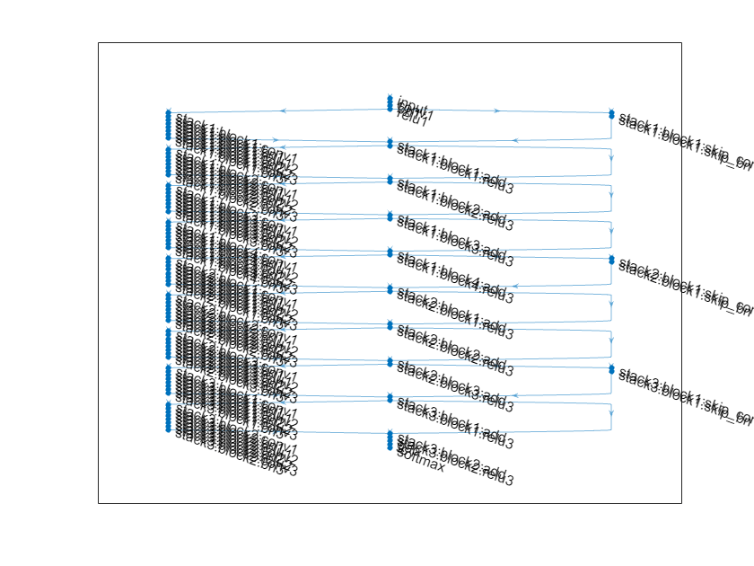
Visualize the network.
plot(net);
Training Options
Specify training options. Train the network for 80 epochs. Select a learning rate that is proportional to the mini-batch size and reduce the learning rate by a factor of 10 after 60 epochs. Validate the network once per epoch using the validation data.
miniBatchSize = 128;
learnRate = 0.1*miniBatchSize/128;
valFrequency = floor(size(XTrain,4)/miniBatchSize);
options = trainingOptions("sgdm", ...
    InitialLearnRate=learnRate, ...
    MaxEpochs=80, ...
    MiniBatchSize=miniBatchSize, ...
    VerboseFrequency=valFrequency, ...
    Shuffle="every-epoch", ...
    Plots="training-progress", ...
    Verbose=false, ...
    ValidationData={XValidation,TValidation}, ...
    ValidationFrequency=valFrequency, ...
    LearnRateSchedule="piecewise", ...
    LearnRateDropFactor=0.1, ...
    LearnRateDropPeriod=60);
Train Network
To train the network using trainnet, set the doTraining flag to true. For classification, use cross-entropy loss. By default, the trainnet function uses a GPU if one is available. Training on a GPU requires a Parallel Computing Toolbox™ license and a supported GPU device. For information on supported devices, see GPU Computing Requirements (Parallel Computing Toolbox). Otherwise, the trainnet function uses the CPU. To specify the execution environment, use the ExecutionEnvironment training option.
Otherwise, load a pretrained network.
doTraining = false;
if doTraining
    net = trainnet(augimdsTrain,net,'crossentropy',options);
else
    load("trainedResidualNetwork.mat","net");
end

Evaluate Trained Network
Calculate the final accuracy of the network on the training set (without data augmentation) and validation set. To make predictions with multiple observations, use the minibatchpredict function. To convert the prediction scores to labels, use the scores2label function. The minibatchpredict function automatically uses a GPU if one is available. Using a GPU requires a Parallel Computing Toolbox™ license and a supported GPU device. For information on supported devices, see GPU Computing Requirements (Parallel Computing Toolbox). Otherwise, the function uses the CPU.
scores = minibatchpredict(net,XValidation);
[YValPred,probs] = scores2label(scores,categories(TValidation));
validationError = mean(YValPred ~= TValidation);
scores = minibatchpredict(net,XTrain);
YTrainPred = scores2label(scores,categories(TTrain));
trainError = mean(YTrainPred ~= TTrain);
disp("Training error: " + trainError*100 + "%")
Training error: 4.168%
disp("Validation error: " + validationError*100 + "%")
Validation error: 9.13%
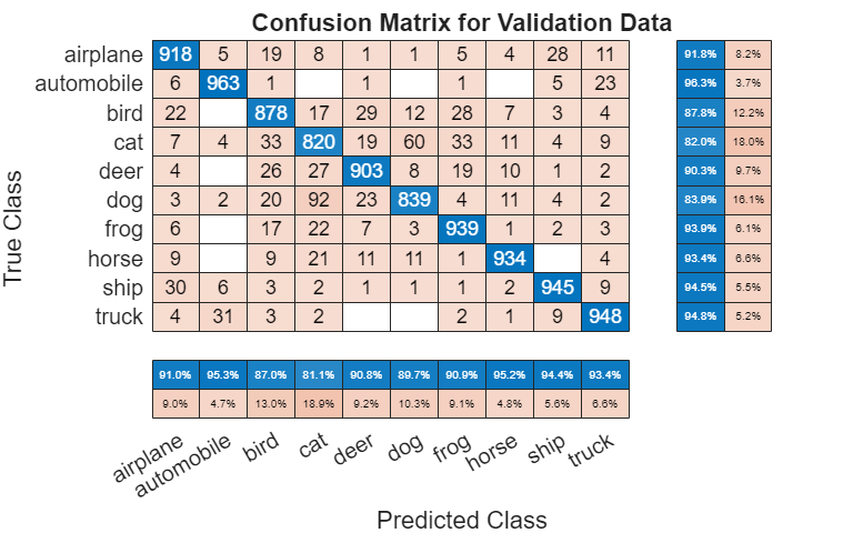
Plot the confusion matrix. Display the precision and recall for each class by using column and row summaries. The network most commonly confuses cats with dogs.
figure(Units="normalized",Position=[0.2 0.2 0.4 0.4]);
cm = confusionchart(TValidation,YValPred);
cm.Title = "Confusion Matrix for Validation Data";
cm.ColumnSummary = "column-normalized";
cm.RowSummary = "row-normalized";
You can display a random sample of nine test images together with their predicted classes and the probabilities of those classes using the following code.
figure
idx = randperm(size(XValidation,4),9);
for i = 1:numel(idx)
    subplot(3,3,i)
    imshow(XValidation(:,:,:,idx(i)));
    prob = num2str(100*max(probs(idx(i),:)),3);
    predClass = char(YValPred(idx(i)));
    title([predClass + ", " + prob + "%"])
end
References
[1] Krizhevsky, Alex. "Learning multiple layers of features from tiny images." (2009). https://www.cs.toronto.edu/~kriz/learning-features-2009-TR.pdf
[2] He, Kaiming, Xiangyu Zhang, Shaoqing Ren, and Jian Sun. "Deep residual learning for image recognition." In Proceedings of the IEEE conference on computer vision and pattern recognition, pp. 770-778. 2016.
See Also
trainnet | trainingOptions | dlnetwork | resnetNetwork | resnet3dNetwork | analyzeNetwork