Training Neural Networks with Tabular Data
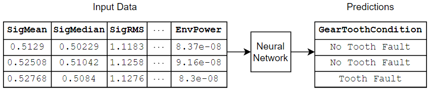
Tabular data refers to data organized into a table with rows that correspond to observations (such as different cars) and columns that correspond to different features of the observations (such as the size and weight of the different cars). You can train a classification neural network to predict categorical labels (such as the car manufacturer) or a regression neural network to predict numerical values (such as the mileage of the cars).
This diagram shows an example of tabular data flowing through a classification neural network that predicts gear faults using transmission casing data.
There are several ways to train neural networks for tabular data:
Train neural network models using Statistics and Machine Learning Toolbox™ — The
fitcnet(Statistics and Machine Learning Toolbox) andfitrnet(Statistics and Machine Learning Toolbox) functions are well suited for most classification and regression neural network tasks, respectively. This is usually the easiest option. For more information, see Train Models for Classification and Regression Using Statistics and Machine Learning Toolbox.Train neural network models using Deep Learning Toolbox™.
Built-in training — The
trainnetfunction is well suited for training with stochastic solvers, such as Adam and SGDM, or training with custom loss functions or neural networks with multiple inputs or outputs. Use this option when you want to customize the training algorithm and loss functions. For more information, see Built-In Training.Custom training loops — If Deep Learning Toolbox does not provide the training options that you need, or you have a model that cannot be defined as a network of layers, then you can define your own custom training loop using automatic differentiation. For more information, see Custom Training Loops.
Train Models for Classification and Regression Using Statistics and Machine Learning Toolbox
To train a classification or regression neural network for tabular data, using the
fitcnet (Statistics and Machine Learning Toolbox) or
fitrnet (Statistics and Machine Learning Toolbox)
functions, respectively, are usually the easiest options. These functions, by default,
train a multilayer perceptron (MLP) neural network. An MLP is a type of neural network
that comprises a series of fully connected layers with activation layers between them.
The fitcnet and fitcnet functions fit the
model using the limited-memory Broyden–Fletcher–Goldfarb–Shanno (L-BFGS) solver, which
is a full-batch solver that processes the entire data set in a single iteration. You can
easily customize aspects of the neural network architecture, such as setting the size
and number of fully connected layers. You can also customize the training algorithm,
such as setting the number of training iterations.
For example, given a table of training data tbl with targets in the
variable responseName, run this command to train a classification
neural
network.
Mdl = fitcnet(tbl,responseName);
If the fitcnet and
fitrnet functions do not provide the functionality for the
network architecture that you need, for example, custom activation functions or
neural networks with skip connections, then you can define the neural network
architecture using a layer array or a dlnetwork object. (since R2025a) This
code shows how to specify a neural network with skip connections and leaky ReLU
layers.
net = dlnetwork;

layers = [
    featureInputLayer(inputSize)
    fullyConnectedLayer(12)
    leakyReluLayer(Name="lrelu1")

    fullyConnectedLayer(12)

    additionLayer(2,Name="add2")
    leakyReluLayer(Name="lrelu2")

    fullyConnectedLayer(12)
    additionLayer(2,Name="add3")
    leakyReluLayer

    fullyConnectedLayer(outputSize)
    softmaxLayer];

net = addLayers(net,layers);
net = connectLayers(net,"lrelu1","add2/in2");
net = connectLayers(net,"lrelu2","add3/in2");

Mdl = fitcnet(tbl,responseName,Network=net);
For a list of available layers, see List of Deep Learning Layers. If Deep Learning Toolbox does not provide the layer that you need, you can define your own layers. For more information, see Define Custom Deep Learning Layers.
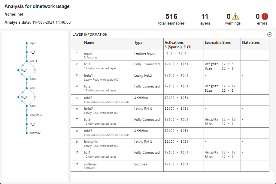
If you train the neural network by specifying a layer array or a
dlnetwork, then to inspect the network architecture and learnable
parameters, convert the model to a dlnetwork object. For example, to
view the neural network architecture and inspect the learnable parameter and activation
sizes, run these
commands.
net = dlnetwork(Mdl);
analyzeNetwork(net);
Train Neural Networks Using Deep Learning Toolbox
Built-In Training
If the fitcnet and fitrnet functions do
not provide the training algorithm options that you need, then using the trainnet with a training options object is usually the easiest
option. For example, use the trainnet function to train with
solvers like Adam and SGDM, or to train with custom loss functions.
To train an simple MLP network using the Adam solver, run these commands.
layers = [
    featureInputLayer(inputSize)
    fullyConnectedLayer(16)
    reluLayer
    fullyConnectedLayer(32)
    reluLayer
    fullyConnectedLayer(outputSize)
    softmaxLayer];

options = trainingOptions("adam");

net = trainnet(tbl,layers,"crossentropy",options);
For an example showing how to train a neural network for tabular data using the
trainnet function, see Train Neural Network with Tabular Data.
Custom Training Loops
If the trainingOptions function does not
provide the training options that you need, for example, a custom solver, then you
can define your own custom training loop using automatic differentiation. For more
information, see Custom Training Loops
For example, to train a neural network with a custom learnable parameter update
function myupdate, run these
commands.
epoch = 0;
iteration = 0;
while epoch < numEpochs
    epoch = epoch + 1;

    reset(mbq);

    while hasdata(mbq)
        iteration = iteration + 1;
        [X,T] = next(mbq);

        [loss,gradients] = dlfeval(lossFcn,net,X,T);

        net = myupdate(net,gradients);
    end
end
For deep learning models that cannot be specified as a neural network of layers, for example, models with loops or conditional branching, you can define your model using a MATLAB® function using automatic differentiation. To train a model defined as a function, use a custom training loop. For more information, see Train Network Using Model Function.
For example, to define a model with a single input and a single output using MATLAB code, you can define a function of this form.
function Y = model(parameters,X)
   ...
end
parameters is an array or structure of
learnable parameters, X is the model input, specified as a
dlarray
object, and Y is the model output.See Also
fitcnet (Statistics and Machine Learning Toolbox) | fitrnet (Statistics and Machine Learning Toolbox) | dlnetwork | trainnet | trainingOptions | dlarray