Brighten Extremely Dark Images Using Deep Learning
This example shows how to recover brightened RGB images from RAW camera data collected in extreme low-light conditions using a U-Net.
Low-light image recovery in cameras is a challenging problem. A typical solution is to increase the exposure time, which allows more light in the scene to hit the sensor and increases the brightness of the image. However, longer exposure times can result in motion blur artifacts when objects in the scene move or when the camera is perturbed during acquisition.
Deep learning offers solutions that recover reasonable images for RAW data collected from DSLRs and many modern phone cameras despite low light conditions and short exposure times. These solutions take advantage of the full information present in RAW data to outperform brightening techniques performed in postprocessed RGB data [1].
Low Light Image (Left) and Recovered Image (Right)

This example shows how to train a network to implement a low-light camera pipeline using data from a particular camera sensor. This example shows how to recover well exposed RGB images from very low light, underexposed RAW data from the same type of camera sensor.
Download See-in-the-Dark Data Set
This example uses the Sony camera data from the See-in-the-Dark (SID) data set [1]. The SID data set provides registered pairs of RAW images of the same scene. In each pair, one image has a short exposure time and is underexposed, and the other image has a longer exposure time and is well exposed. The size of the Sony camera data from the SID data set is 25 GB.
Set dataDir as the desired location of the data set.
dataDir = fullfile(tempdir,"SID");To download the data set, go to this link: https://storage.googleapis.com/isl-datasets/SID/Sony.zip. Extract the data into the directory specified by the dataDir variable. When extraction is successful, dataDir contains the directory Sony with two subdirectories: long and short. The files in the long subdirectory have a long exposure and are well exposed. The files in the short subdirectory have a short exposure and are quite underexposed and dark.
The data set also provides text files that describe how to partition the files into training, validation, and test data sets. Move the files Sony_train_list.txt, Sony_val_list.txt, and Sony_test_list.txt to the directory specified by the dataDir variable.
Import the list of files to include in the training, validation, and test data sets using the importSonyFileInfo helper function. This function is attached to the example as a supporting file.
trainInfo = importSonyFileInfo(fullfile(dataDir,"Sony_train_list.txt"));
valInfo = importSonyFileInfo(fullfile(dataDir,"Sony_val_list.txt"));
testInfo = importSonyFileInfo(fullfile(dataDir,"Sony_test_list.txt"));
Create Datastores for Training, Validation, and Testing
Combine and Preprocess RAW and RGB Data Using Datastores
Create combined datastores that read and preprocess pairs of underexposed and well exposed RAW images using the createCombinedDatastoreForLowLightRecovery helper function. This function is attached to the example as a supporting file.
The createCombinedDatastoreForLowLightRecovery helper function performs these operations:
Create an
imageDatastorethat reads the short exposure RAW images using a custom read function. The read function reads a RAW image using therawread(Image Processing Toolbox) function, then separates the RAW Bayer pattern into separate channels for each of the four sensors using theraw2planar(Image Processing Toolbox) function. Normalize the data to the range [0, 1] by transforming theimageDatastoreobject.Create an
imageDatastoreobject that reads long-exposure RAW images and converts the data to an RGB image in one step using theraw2rgb(Image Processing Toolbox) function. Normalize the data to the range [0, 1] by transforming theimageDatastoreobject.Combine the
imageDatastoreobjects using thecombinefunction.Apply a simple multiplicative gain to the pairs of images. The gain corrects for the exposure time difference between the shorter exposure time of the dark inputs and the longer exposure time of the output images. This gain is defined by taking the ratio of the long and short exposure times provided in the image file names.
Associate the images with metadata such as exposure time, ISO, and aperture.
dsTrainFull = createCombinedDatastoreForLowLightRecovery(dataDir,trainInfo);
dsValFull = createCombinedDatastoreForLowLightRecovery(dataDir,valInfo);
dsTestFull = createCombinedDatastoreForLowLightRecovery(dataDir,testInfo);
The testing data set does not require preprocessing. Test images are fed at full size into the network.
Preprocess Training Data
Define a helper function called extractRandomPatch that preprocesses training data. The extractRandomPatch helper function crops multiple random patches from a planar RAW image and corresponding patches from an RGB image. The RAW data patch has size m-by-n-by-4 and the RGB image patch has size 2m-by-2n-by-3, where [m n] is the value of the targetRAWSize input argument. Both patches have the same scene content.
function dataOut = extractRandomPatch(data,targetRAWSize,patchesPerImage)
    dataOut = cell(patchesPerImage,2);
    raw = data{1};
    rgb = data{2};
    for idx = 1:patchesPerImage
        windowRAW = randomCropWindow3d(size(raw),targetRAWSize);
        windowRGB = images.spatialref.Rectangle( ...
            2*windowRAW.XLimits+[-1,0],2*windowRAW.YLimits+[-1,0]);
        dataOut(idx,:) = {imcrop3(raw,windowRAW),imcrop(rgb,windowRGB)};
    end
end
Preprocess the training data set using the transform function and the extractRandomPatch helper function. Crop patches of size 512-by-512-by-4 pixels from a planar RAW image and corresponding patches of size 1024-by-1024-by-3 pixels from an RGB image. Extract 12 patches per training image.
inputSize = [512,512,4];
patchesPerImage = 12;
dsTrain = transform(dsTrainFull, ...
    @(data) extractRandomPatch(data,inputSize,patchesPerImage));
Preview an original full-sized image and a random training patch.
previewFull = preview(dsTrainFull);
previewPatch = preview(dsTrain);
montage({previewFull{1,2},previewPatch{1,2}},BackgroundColor="w");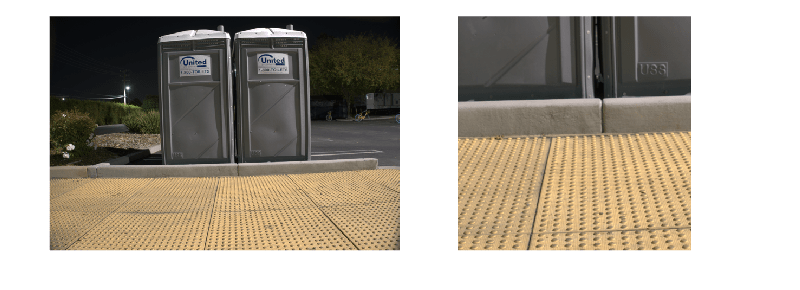
Augment Training Data
Augment the training data set using the transform function and the augmentPatchesForLowLightRecovery helper function. This function is attached to the example as a supporting file. The augmentPatchesForLowLightRecovery helper function adds random horizontal and vertical reflection and randomized 90-degree rotations to pairs of training image patches.
dsTrain = transform(dsTrain,@(data) augmentPatchesForLowLightRecovery(data));
Verify that the preprocessing and augmentation operations work as expected by previewing one channel from the planar RAW image patch and the corresponding RGB decoded patch. The planar RAW data and the target RGB data depict patches of the same scene, randomly extracted from the original source image. Significant noise is visible in the RAW patch because of the short acquisition time of the RAW data, causing a low signal-to-noise ratio.
imagePairs = read(dsTrain);
rawImage = imagePairs{1,1};
rgbPatch = imagePairs{1,2};
montage({rawImage(:,:,1),rgbPatch});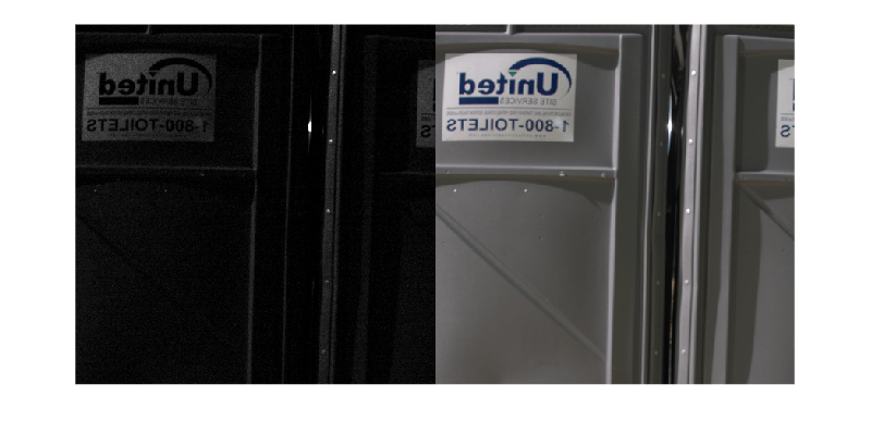
Preprocess Validation Data
Use a subset of the validation images to make computation of validation metrics quicker.
numVal = 30;
dsValFull = shuffle(dsValFull);
dsVal = subset(dsValFull,1:numVal);
Define a helper function called extractCenterPatch that preprocesses validation data. The extractCenterPatch helper function crops a single patch from the center of a planar RAW image and the corresponding patch from an RGB image. The RAW data patch has size m-by-n-by-4 and the RGB image patch has size 2m-by-2n-by-3, where [m n] is the value of the targetRAWSize input argument. Both patches have the same scene content.
function dataOut = extractCenterPatch(data,targetRAWSize)
    raw = data{1};
    rgb = data{2};
    windowRAW = centerCropWindow3d(size(raw),targetRAWSize);
    windowRGB = images.spatialref.Rectangle( ...
        2*windowRAW.XLimits+[-1,0],2*windowRAW.YLimits+[-1,0]);
    dataOut = {imcrop3(raw,windowRAW),imcrop(rgb,windowRGB)};
end
Preprocess the validation data set using the transform function and the extractCenterPatch helper function. Crop a patch of size 512-by-512-by-4 pixels from the center of a planar RAW image and a corresponding patch of size 1024-by-1024-by-3 pixels from an RGB image.
dsVal = transform(dsVal,@(data) extractCenterPatch(data,inputSize));
Define Network
Use a network architecture similar to U-Net. The example creates the encoder and decoder subnetworks using the blockedNetwork (Image Processing Toolbox) function. This function creates the encoder and decoder subnetworks programmatically using the buildEncoderBlock and buildDecoderBlock helper functions, respectively. The helper functions are defined at the end of this example. The example uses instance normalization between convolution and activation layers in all network blocks except the first and last, and uses a leaky ReLU layer as the activation layer.
Create an encoder subnetwork that consists of four encoder modules. The first encoder module has 32 channels, or feature maps. Each subsequent module doubles the number of feature maps from the previous encoder module.
numModules = 4;
numChannelsEncoder = 2.^(5:8);
encoder = blockedNetwork(@(block) buildEncoderBlock(block,numChannelsEncoder), ...
    numModules,NamePrefix="encoder");
Create a decoder subnetwork that consists of four decoder modules. The first decoder module has 256 channels, or feature maps. Each subsequent decoder module halves the number of feature maps from the previous decoder module.
numChannelsDecoder = fliplr(numChannelsEncoder);
decoder = blockedNetwork(@(block) buildDecoderBlock(block,numChannelsDecoder), ...
    numModules,NamePrefix="decoder");
Specify the bridge layers that connect the encoder and decoder subnetworks.
bridgeLayers = [
    convolution2dLayer(3,512,Padding="same",PaddingValue="replicate")
    groupNormalizationLayer("channel-wise")
    leakyReluLayer(0.2)
    convolution2dLayer(3,512,Padding="same",PaddingValue="replicate")
    groupNormalizationLayer("channel-wise")
    leakyReluLayer(0.2)];
Specify the final layers of the network.
finalLayers = [
    convolution2dLayer(1,12)
    depthToSpace2dLayer(2)];
Combine the encoder subnetwork, bridge layers, decoder subnetwork, and final layers using the encoderDecoderNetwork (Image Processing Toolbox) function.
net = encoderDecoderNetwork(inputSize,encoder,decoder, ...
    LatentNetwork=bridgeLayers, ...
    SkipConnections="concatenate", ...
    FinalNetwork=finalLayers);
Use mean centering normalization on the input as part of training.
net = replaceLayer(net,"encoderImageInputLayer", ...
    imageInputLayer(inputSize,Normalization="zerocenter"));
Define Loss Function
Define a custom loss function called lossFcn that calculates an overall loss during training. The overall loss is a weighted sum of two losses:
function loss = lossFcn(Y,T)
    ssimLoss = mean(1-multissim(rgbToGray(Y),rgbToGray(T),NumScales=5),"all");
    L1loss =  mean(abs(Y-T),"all");

    alpha = 7/8;
    loss = alpha*ssimLoss + (1-alpha)*L1loss;
end
Specify Training Options
For training, use the Adam solver with an initial learning rate of 1e-3. Train for 30 epochs.
miniBatchSize = 12;
maxEpochs = 30;
options = trainingOptions("adam", ...
    Plots="training-progress", ...
    MiniBatchSize=miniBatchSize, ...
    InitialLearnRate=1e-3, ...
    MaxEpochs=maxEpochs, ...
    ValidationFrequency=400);
Train Network or Download Pretrained Network
By default, the example loads a pretrained version of the low-light recovery network. The pretrained network enables you to run the entire example without waiting for training to complete.
To train the network, set the doTraining variable in the following code to true. Train the model using the trainnet function. Specify the loss function as lossFcn. By default, the trainnet function uses a GPU if one is available. Training on a GPU requires a Parallel Computing Toolbox™ license and a supported GPU device. For information on supported devices, see GPU Computing Requirements (Parallel Computing Toolbox). Otherwise, the trainnet function uses the CPU. To specify the execution environment, use the ExecutionEnvironment training option.
doTraining = false;

if doTraining
    checkpointsDir = fullfile(dataDir,"checkpoints");
    if ~exist(checkpointsDir,"dir")
        mkdir(checkpointsDir);
    end
    options.CheckpointPath=checkpointsDir;

    netTrained = trainnet(dsTrain,net,@lossFcn,options);
    modelDateTime = string(datetime("now",Format="yyyy-MM-dd-HH-mm-ss"));
    save(fullfile(dataDir,"trainedLowLightCameraPipelineNet-"+modelDateTime+".mat"), ...
        "netTrained");

else
    trainedNet_url = "https://ssd.mathworks.com/supportfiles/"+ ...
        "vision/data/trainedLowLightCameraPipelineDlnetwork.zip";
    downloadTrainedNetwork(trainedNet_url,dataDir);
    load(fullfile(dataDir,"trainedLowLightCameraPipelineNet.mat"));
end
Examine Results from Trained Network
Visually examine the results of the trained low-light camera pipeline network.
Read a pair of images and accompanying metadata from the test set. Get the file names of the short and long exposure images from the metadata.
[testPair,info] = read(dsTestFull);
testShortFilename = info.ShortExposureFilename;
testLongFilename = info.LongExposureFilename;
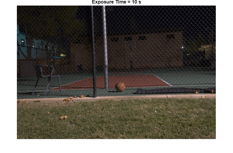
Convert the original underexposed RAW image to an RGB image in one step using the raw2rgb (Image Processing Toolbox) function. Display the result, scaling the display range to the range of pixel values. The image looks almost completely black, with only a few bright pixels.
testShortImage = raw2rgb(testShortFilename);
testShortTime = info.ShortExposureTime;
imshow(testShortImage,[])
title("Exposure Time = "+num2str(testShortTime)+" s")

Convert the original well exposed RAW image to an RGB image in one step using the raw2rgb (Image Processing Toolbox) function. Display the result.
testLongImage = raw2rgb(testLongFilename);
testLongTime = info.LongExposureTime;
imshow(testLongImage)
title("Exposure Time = "+num2str(testLongTime)+" s")
Display the network prediction. The trained network recovers an impressive image under challenging acquisition conditions with very little noise or other visual artifacts. The colors of the network prediction are less saturated and vibrant than in the ground truth long-exposure image of the scene.
inputImage = dlarray(testPair{1},"SSCB");
if canUseGPU
    inputImage = gpuArray(inputImage);
end

outputFromNetwork = gather(extractdata(predict(netTrained,inputImage)));
outputFromNetwork = im2uint8(outputFromNetwork);

imshow(outputFromNetwork)
title("Low-Light Recovery Network Prediction")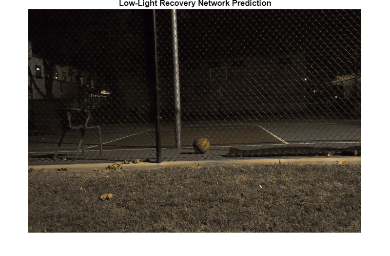
Supporting Functions
The buildEncoderBlock helper function defines the layers of a single encoder module within the encoder subnetwork.
function block = buildEncoderBlock(blockIdx,numChannelsEncoder)

    if blockIdx < 2
        instanceNorm = [];
    else
        instanceNorm = instanceNormalizationLayer;
    end

    filterSize = 3;
    numFilters = numChannelsEncoder(blockIdx);
    block = [
        convolution2dLayer(filterSize,numFilters,Padding="same", ...
            PaddingValue="replicate",WeightsInitializer="he")
        instanceNorm
        leakyReluLayer(0.2)
        convolution2dLayer(filterSize,numFilters,Padding="same", ...
            PaddingValue="replicate",WeightsInitializer="he")
        instanceNorm
        leakyReluLayer(0.2)
        maxPooling2dLayer(2,Stride=2,Padding="same")];
end
The buildDecoderBlock helper function defines the layers of a single encoder module within the decoder subnetwork.
function block = buildDecoderBlock(blockIdx,numChannelsDecoder)

    if blockIdx < 4
        instanceNorm = instanceNormalizationLayer;
    else
        instanceNorm = [];
    end

    filterSize = 3;
    numFilters = numChannelsDecoder(blockIdx);
    block = [
        transposedConv2dLayer(filterSize,numFilters,Stride=2, ...
            WeightsInitializer="he",Cropping="same")
        convolution2dLayer(filterSize,numFilters,Padding="same", ...
            PaddingValue="replicate",WeightsInitializer="he")
        instanceNorm
        leakyReluLayer(0.2)
        convolution2dLayer(filterSize,numFilters,Padding="same", ...
            PaddingValue="replicate",WeightsInitializer="he")
        instanceNorm
        leakyReluLayer(0.2)];
end
The rgbToGray helper function converts a batch of RGB images to grayscale. The grayscale channel is a linear combination of the red, green, and blue channels according to: Y = 0.2989*R + 0.5810*G + 0.1140*B.
function y = rgbToGray(rgb)
    sizeIn = size(rgb,[1 2]);
    batchSize = size(rgb,4);
    weights = [0.2989; 0.5810; 0.1140];
    rgb = reshape(rgb,[],size(rgb,3),size(rgb,4));
    y = pagemtimes(rgb,weights);
    y = reshape(y,[sizeIn,1,batchSize]);
end
References
[1] Chen, Chen, Qifeng Chen, Jia Xu, and Vladlen Koltun. "Learning to See in the Dark." Preprint, submitted May 4, 2018. https://arxiv.org/abs/1805.01934.
See Also
trainnet | trainingOptions | dlnetwork | predict | imageDatastore | transform | combine
Related Examples
More About
Select a Web Site
Choose a web site to get translated content where available and see local events and offers. Based on your location, we recommend that you select: United States.
You can also select a web site from the following list
Americas
- América Latina (Español)
- Canada (English)
- United States (English)
Europe
- Belgium (English)
- Denmark (English)
- Deutschland (Deutsch)
- España (Español)
- Finland (English)
- France (Français)
- Ireland (English)
- Italia (Italiano)
- Luxembourg (English)
- Netherlands (English)
- Norway (English)
- Österreich (Deutsch)
- Portugal (English)
- Sweden (English)
- Switzerland
- United Kingdom (English)
Asia Pacific
- Australia (English)
- India (English)
- New Zealand (English)
- 中国
- 日本Japanese (日本語)
- 한국Korean (한국어)