plotconfusion
(To be removed) Plot classification confusion matrix
plotconfusion will be removed in a future release. For more information,
see Transition Legacy Neural Network Code to dlnetwork Workflows.
For advice on updating your code, see Version History.
Syntax
Description
plotconfusion(
plots a confusion matrix for the true labels targets,outputs)targets and
predicted labels outputs. Specify the labels as categorical
vectors, or in one-of-N (one-hot) form.
Tip
plotconfusion is not recommended for categorical
labels. Use confusionchart instead.
On the confusion matrix plot, the rows correspond to the predicted class (Output Class) and the columns correspond to the true class (Target Class). The diagonal cells correspond to observations that are correctly classified. The off-diagonal cells correspond to incorrectly classified observations. Both the number of observations and the percentage of the total number of observations are shown in each cell.
The column on the far right of the plot shows the percentages of all the examples predicted to belong to each class that are correctly and incorrectly classified. These metrics are often called the precision (or positive predictive value) and false discovery rate, respectively. The row at the bottom of the plot shows the percentages of all the examples belonging to each class that are correctly and incorrectly classified. These metrics are often called the recall (or true positive rate) and false negative rate, respectively. The cell in the bottom right of the plot shows the overall accuracy.
plotconfusion(targets1,outputs1,name1,targets2,outputs2,name2,...,targetsn,outputsn,namen)
plots multiple confusion matrices in one figure and adds the
name arguments to the beginnings of the titles of the
corresponding plots.
Examples
Load the data consisting of synthetic images of handwritten digits. XTrain is a 28-by-28-by-1-by-5000 array of images and labelsTrain is a categorical vector containing the image labels.
load DigitsDataTrain
classNames = categories(labelsTrain);
Define the architecture of a convolutional neural network.
layers = [
    imageInputLayer([28 28 1])

    convolution2dLayer(3,8,'Padding','same')
    batchNormalizationLayer
    reluLayer
    convolution2dLayer(3,16,'Padding','same','Stride',2)
    batchNormalizationLayer
    reluLayer
    convolution2dLayer(3,32,'Padding','same','Stride',2)
    batchNormalizationLayer
    reluLayer

    fullyConnectedLayer(10)
    softmaxLayer];
Specify training options and train the network.
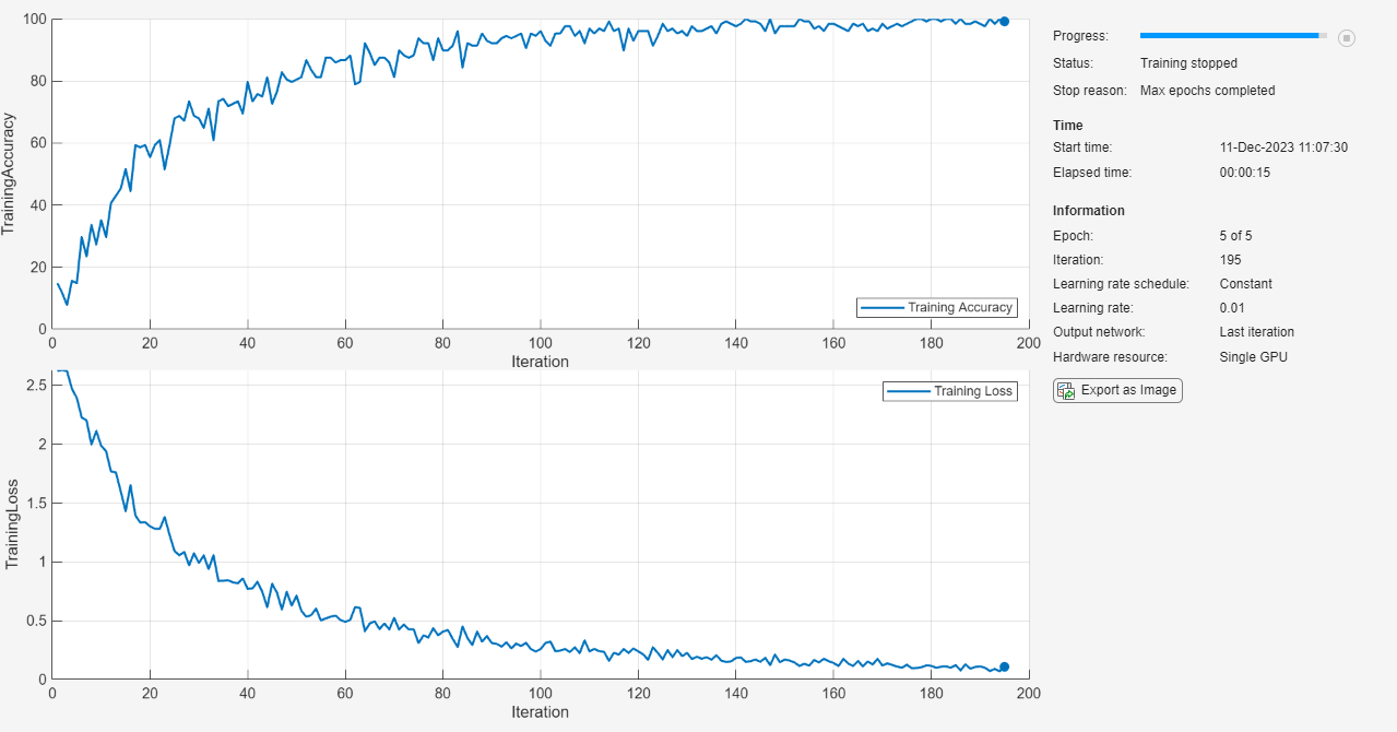
options = trainingOptions('sgdm', ...
    'MaxEpochs',5, ...
    'Verbose',false, ...
    'Plots','training-progress', ...
    'Metrics','accuracy');
net = trainnet(XTrain,labelsTrain,layers,"crossentropy",options);
Load and classify test data using the trained network.
load DigitsDataTest
scores = minibatchpredict(net,XTest);
YTest = scores2label(scores,classNames);
Plot the confusion matrix of the test labels and the predicted labels.
plotconfusion(labelsTest,YTest)
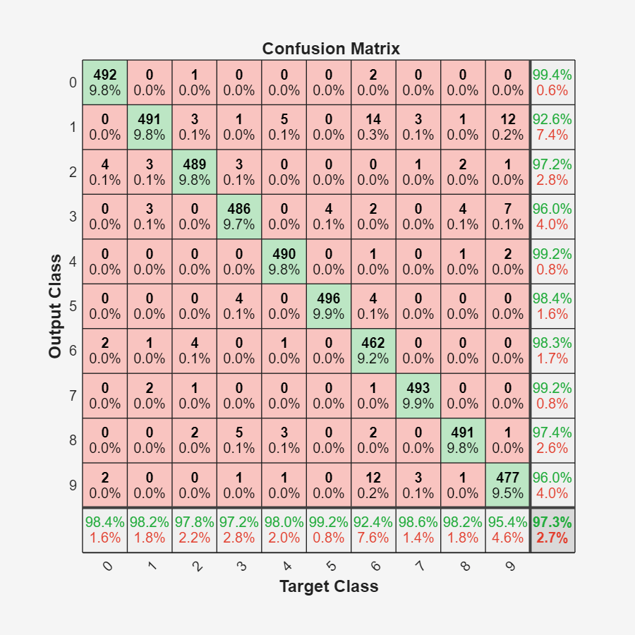
The rows correspond to the predicted class (Output Class) and the columns correspond to the true class (Target Class). The diagonal cells correspond to observations that are correctly classified. The off-diagonal cells correspond to incorrectly classified observations. Both the number of observations and the percentage of the total number of observations are shown in each cell.
The column on the far right of the plot shows the percentages of all the examples predicted to belong to each class that are correctly and incorrectly classified. These metrics are often called the precision (or positive predictive value) and false discovery rate, respectively. The row at the bottom of the plot shows the percentages of all the examples belonging to each class that are correctly and incorrectly classified. These metrics are often called the recall (or true positive rate) and false negative rate, respectively. The cell in the bottom right of the plot shows the overall accuracy.
Close all figures.
close(findall(groot,'Type','figure'))
Input Arguments
Version History
Introduced in R2008aSee Also
confusionchart | Time Series
Modeler | fitrnet (Statistics and Machine Learning Toolbox) | fitcnet (Statistics and Machine Learning Toolbox) | trainnet | trainingOptions | dlnetwork