taylorPrunableNetwork

Network that can be pruned by using first-order Taylor approximation

Since R2022a

Description

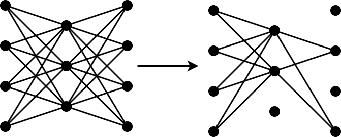
A TaylorPrunableNetwork object enables support for pruning of filters in convolution layers by using first-order Taylor approximation. To prune filters in a dlnetwork object, first convert it to a TaylorPrunableNetwork object and then use the associated object functions.

To prune a deep neural network, you require the Deep Learning Toolbox™ Model Quantization Library support package. This support package is a free add-on that you can download using the Add-On Explorer. Alternatively, see Deep Learning Toolbox Model Quantization Library.

Creation

Syntax

prunableNet = taylorPrunableNetwork(net)

Description

prunableNet = taylorPrunableNetwork(net) converts the specified neural network to a TaylorPrunableNetwork object. A TaylorPrunableNetwork is a different representation of the same network that is suitable for pruning by using the Taylor pruning algorithm. If the input network does not support pruning, then the function throws an error.

Input Arguments

net — Neural network architecture

dlnetwork object | layer array

Neural network architecture, specified as a dlnetwork object or a layer array.

For a list of built-in neural network layers, see List of Deep Learning Layers.

Properties

Learnables — Network learnable parameters

table

Network learnable parameters, specified as a table with three columns:

• Layer — Layer name, specified as a string scalar.

• Parameter — Parameter name, specified as a string scalar.

• Value — Value of parameter, specified as a dlarray object.

The network learnable parameters contain the features learned by the network. For example, the weights of convolution and fully connected layers.

The learnable parameter values can be complex-valued. (since R2024a)

Data Types: table

State — Network state

table

Network state, specified as a table.

The network state is a table with three columns:

• Layer – Layer name, specified as a string scalar.

• Parameter – State parameter name, specified as a string scalar.

• Value – Value of state parameter, specified as a dlarray object.

Layer states contain information calculated during the layer operation to be retained for use in subsequent forward passes of the layer. For example, the cell state and hidden state of LSTM layers, or running statistics in batch normalization layers.

For recurrent layers, such as LSTM layers, with the HasStateInputs property set to 1 (true), the state table does not contain entries for the states of that layer.

During training or inference, you can update the network state using the output of the forward and predict functions.

The state values can be complex-valued. (since R2024a)

Data Types: table

InputNames — Names of network inputs

cell array of character vectors

This property is read-only.

Names of the network inputs, specified as a cell array of character vectors.

Network inputs are the input layers and the unconnected inputs of layers.

For input layers and layers with a single input, the input name is the name of the layer. For layers with multiple inputs, the input name is "layerName/inputName", where layerName is the name of the layer and inputName is the name of the layer input.

Data Types: cell

OutputNames — Names of network outputs

cell array of character vectors

Names of the network outputs, specified as a cell array of character vectors.

For layers with a single output, the output name is the name of the layer. For layers with multiple outputs, the output name is "layerName/outputName", where layerName is the name of the layer and outputName is the name of the layer output.

If you do not specify the output names, then the software sets the OutputNames property to the layers with unconnected outputs.

The predict and forward functions, by default, return the data output by the layers given by the OutputNames property.

Data Types: cell

NumPrunables — Number of convolution layer filters that are suitable for pruning

nonnegative integer

Number of convolution layer filters in the network that are suitable for pruning by using first-order Taylor approximation, specified as a nonnegative integer.

Object Functions

forward	Compute deep learning network output for training
predict	Compute deep learning network output for inference
updatePrunables	Remove filters from prunable layers based on importance scores
updateScore	Compute and accumulate Taylor-based importance scores for pruning
dlnetwork	Deep learning neural network

Examples

Prune dlnetwork Object to Compress the Model

This example shows how to prune a dlnetwork object by using a custom pruning loop.

Load dlnetwork Object

Load a trained dlnetwork object and the corresponding classes.

s = load("digitsCustom.mat");
dlnet_1 = s.dlnet;
classes = s.classes;

Inspect the layers of the dlnetwork object. The network has three convolution layers at locations 2, 5, and 8 of the Layer array.

layers_1 = dlnet_1.Layers

layers_1 = 
  12x1 Layer array with layers:

     1   'input'     Image Input           28x28x1 images with 'zerocenter' normalization
     2   'conv1'     2-D Convolution       20 5x5x1 convolutions with stride [1  1] and padding [0  0  0  0]
     3   'bn1'       Batch Normalization   Batch normalization with 20 channels
     4   'relu1'     ReLU                  ReLU
     5   'conv2'     2-D Convolution       20 3x3x20 convolutions with stride [1  1] and padding [1  1  1  1]
     6   'bn2'       Batch Normalization   Batch normalization with 20 channels
     7   'relu2'     ReLU                  ReLU
     8   'conv3'     2-D Convolution       20 3x3x20 convolutions with stride [1  1] and padding [1  1  1  1]
     9   'bn3'       Batch Normalization   Batch normalization with 20 channels
    10   'relu3'     ReLU                  ReLU
    11   'fc'        Fully Connected       10 fully connected layer
    12   'softmax'   Softmax               softmax

Load Data for Prediction

Load the digits data for prediction.

dataFolder = fullfile(toolboxdir("nnet"),"nndemos","nndatasets","DigitDataset");

imds = imageDatastore(dataFolder, ...
    IncludeSubfolders=true, ...
    LabelSource="foldernames");

Partition the data into pruning and validation sets. Set aside 10% of the data for validation using the splitEachLabel function.

[imdsPrune,imdsValidation] = splitEachLabel(imds,0.9,"randomize");

The network used in this example requires input images of size 28-by-28-by-1. To automatically resize the images, use augmented image datastores.

inputSize = [28 28 1];
augimdsPrune = augmentedImageDatastore(inputSize(1:2),imdsPrune);
augimdsValidation = augmentedImageDatastore(inputSize(1:2),imdsValidation);

Prune dlnetwork Object

Convert the dlnetwork object to a representation that is suitable for pruning by using the taylorPrunableNetwork function. This function returns a TaylorPrunableNetwork object that has the NumPrunables property set to 48. This indicates that 48 filters in the original model are suitable for pruning by using the Taylor pruning algorithm.

prunableNet_1 = taylorPrunableNetwork(dlnet_1)

prunableNet_1 = 
  TaylorPrunableNetwork with properties:

      Learnables: [14x3 table]
           State: [6x3 table]
      InputNames: {'input'}
     OutputNames: {'softmax'}
    NumPrunables: 48

Create a minibatchqueue object that processes and manages mini-batches of images during pruning. For each mini-batch:

• Use the custom mini-batch preprocessing function preprocessMiniBatch (defined at the end of this example) to convert the labels to one-hot encoded variables.

• Format the image data with the dimension labels "SSCB" (spatial, spatial, channel, batch). By default, the minibatchqueue object converts the data to dlarray objects with underlying type single. Do not format the class labels.

• Train on a GPU if one is available. By default, the minibatchqueue object converts each output to a gpuArray if a GPU is available. Using a GPU requires Parallel Computing Toolbox™ and a supported GPU device. For information on supported devices, see GPU Computing Requirements (Parallel Computing Toolbox).

miniBatchSize = 128;
imds.ReadSize = miniBatchSize;

mbq = minibatchqueue(augimdsPrune, ...
    MiniBatchSize=miniBatchSize, ...
    MiniBatchFcn=@preprocessMiniBatch, ...
    MiniBatchFormat=["SSCB" ""]);

Calculate Taylor-based importance scores of the prunable filters in the network by looping over the mini-batches of data. For each mini-batch:

• Calculate pruning activations and pruning gradients by using the modelLoss function defined at the end of this example

• Update importance scores of the prunable filters by using the updateScore function

while hasdata(mbq)
    [X,T] = next(mbq);
    [~,pruningActivations,pruningGradients] = dlfeval(@modelLoss,prunableNet_1,X,T);
    prunableNet_1 = updateScore(prunableNet_1,pruningActivations,pruningGradients);
end

Finally, remove filters with the lowest importance scores to create a new TaylorPrunableNetwork object by using the updatePrunables function. By default, a single call to this function removes 8 filters. Observe that the new network prunableNet_2 has 40 prunable filters remaining.

prunableNet_2 = updatePrunables(prunableNet_1)

prunableNet_2 = 
  TaylorPrunableNetwork with properties:

      Learnables: [14x3 table]
           State: [6x3 table]
      InputNames: {'input'}
     OutputNames: {'softmax'}
    NumPrunables: 40

To further compress the model, run the custom pruning loop and update prunables again.

Extract Pruned dlnetwork Object

Use the dlnetwork function to extract the pruned dlnetwork object from the pruned TaylorPrunableNetwork object. You can now use this compressed dlnetwork object to perform inference.

dlnet_2 = dlnetwork(prunableNet_2);

Compare the convolution layers of the original and the pruned dlnetwork objects. Observe that the three convolution layers in the pruned network have fewer filters. These counts agree with the fact that, by default, a single call to the updatePrunables function removes 8 filters from the network.

conv_layers_1 = dlnet_1.Layers([2 5 8])

conv_layers_1 = 
  3x1 Convolution2DLayer array with layers:

     1   'conv1'   2-D Convolution   20 5x5x1 convolutions with stride [1  1] and padding [0  0  0  0]
     2   'conv2'   2-D Convolution   20 3x3x20 convolutions with stride [1  1] and padding [1  1  1  1]
     3   'conv3'   2-D Convolution   20 3x3x20 convolutions with stride [1  1] and padding [1  1  1  1]

conv_layers_2 = dlnet_2.Layers([2 5 8])

conv_layers_2 = 
  3x1 Convolution2DLayer array with layers:

     1   'conv1'   2-D Convolution   17 5x5x1 convolutions with stride [1  1] and padding [0  0  0  0]
     2   'conv2'   2-D Convolution   18 3x3x17 convolutions with stride [1  1] and padding [1  1  1  1]
     3   'conv3'   2-D Convolution   17 3x3x18 convolutions with stride [1  1] and padding [1  1  1  1]

Supporting Functions

Model Loss Function

The modelLoss function takes a TaylorPrunableNetwork object net, a mini-batch of input data X with corresponding targets T and returns activations in net and the gradients of the loss with respect to the activations in net. To compute the gradients automatically, this function uses the dlgradient function.

function [loss, pruningActivations, pruningGradients] = modelLoss(net,X,T)

% Calculate network output for training.
[out, ~, pruningActivations] = forward(net,X);

% Calculate loss.
loss = crossentropy(out,T);

% Compute pruning gradients.
pruningGradients = dlgradient(loss,pruningActivations);
end

Mini Batch Preprocessing Function

The preprocessMiniBatch function preprocesses a mini-batch of predictors and labels using the following steps:

1. Preprocess the images using the preprocessMiniBatchPredictors function.

2. Extract the label data from the incoming cell array and concatenate into a categorical array along the second dimension.

3. One-hot encode the categorical labels into numeric arrays. Encoding into the first dimension produces an encoded array that matches the shape of the network output.

function [X,T] = preprocessMiniBatch(dataX,dataT)

% Preprocess predictors.
X = preprocessMiniBatchPredictors(dataX);

% Extract label data from cell and concatenate.
T = cat(2,dataT{1:end});

% One-hot encode labels.
T = onehotencode(T,1);

end

Mini-Batch Predictors Preprocessing Function

The preprocessMiniBatchPredictors function preprocesses a mini-batch of predictors by extracting the image data from the input cell array and concatenating into a numeric array. For grayscale input, concatenating over the fourth dimension adds a third dimension to each image, to use as a singleton channel dimension.

function X = preprocessMiniBatchPredictors(dataX)

% Concatenate.
X = cat(4,dataX{1:end});

% Normalize the images.
X = X/255;

end

Analyze Taylor Prunable Network

Load a trained and pruned taylorPrunableNetwork object.

load("prunedDigitsCustom.mat");

Analyze the network. analyzeNetwork displays an interactive plot of the network architecture and a table containing information about the network layers. The table shows the number of pruned convolutional filters. The table also shows the percentage decrease in the number of learnables for each layer. This includes the three convolutional layers, but also downstream effects in other layers that do not have pruned filters.

analyzeNetwork(prunableNet)

More About

Layers Supported for Pruning

The Taylor pruning algorithm prunes filters from convolution2dLayer objects. Pruning convolutional filters can also reduce the number of learnable parameters in downstream layers, for example:

• batchNormalizationLayer

• fullyConnectedLayer

• groupedConvolution2dLayer

• transposedConv2dLayer

Effect of Network Architecture on Pruning

For certain network architectures, data dependency between the prunable layers and other layers in the network might prevent pruning of filters. These are some example architectures that exhibit this behavior:

• Your network has a convolution2dLayer, a groupNormalizationLayer and another convolution2dLayer connected in sequence. The presence of the group normalization layer prevents pruning of filters of the first convolution layer, because doing so changes the shape of the input channels of the group normalization layer.

• Your network has a 2-D convolution layer, a softmax layer, and an output layer connected in sequence. This architecture prevents pruning of filters of the convolution layer because doing so changes the output size of the network.

Algorithms

For an individual input data point in the pruning dataset, you use the forward function to calculate the output of the deep learning network and the activations of the prunable filters. Then you calculate the gradients of the loss with respect to these activations using automatic differentiation. You then pass the network, the activations, and the gradients to the updateScore function. For each prunable filter in the network, the updateScore function calculates the change in loss that occurs if that filter is pruned from the network (up to first-order Taylor approximation). Based on this change, the function associates an importance score with that filter and updates the TaylorPrunableNetwork object [1].

Inside the custom pruning loop, you accumulate importance scores for the prunable filters over all mini-batches of the pruning dataset. Then you pass the network object to the updatePrunables function. This functions prunes the filters that have the lowest importance scores and hence have the smallest effect on the accuracy of the network output. The number of filters that a single call to the updatePrunables function prunes is determined by the optional name-value argument MaxToPrune, that has a default value of 8.

All these steps complete a single pruning iteration. To further compress your model, repeat these steps multiple times over a loop.

References

[1] Molchanov, Pavlo, Stephen Tyree, Tero Karras, Timo Aila, and Jan Kautz. "Pruning Convolutional Neural Networks for Resource Efficient Inference." Preprint, submitted June 8, 2017. https://arxiv.org/abs/1611.06440.

Version History

Introduced in R2022a

R2024a: Complex-valued learnables and state

The values in the Learnables and State properties can be complex-valued.

R2024a: LayerGraph objects are not recommended

Starting in R2024a, LayerGraph objects are not recommended. Use dlnetwork objects instead. This recommendation means that LayerGraph input is not recommended to the taylorPrunableNetwork function.

Most functions that support LayerGraph objects also support dlnetwork objects. This table shows some typical usages of LayerGraph objects and how to update your code to use dlnetwork object functions instead.

Not Recommended	Recommended
lgraph = layerGraph;	net = dlnetwork;
lgraph = layerGraph(layers);	net = dlnetwork(layers,Initialize=false);
lgraph = layerGraph(net);	net = dag2dlnetwork(net);
lgraph = addLayers(lgraph,layers);	net = addLayers(net,layers);
lgraph = removeLayers(lgraph,layerNames);	net = removeLayers(net,layerNames);
lgraph = replaceLayer(lgraph,layerName,layers);	net = replaceLayer(net,layerName,layers);
lgraph = connectLayers(lgraph,s,d);	net = connectLayers(net,s,d);
lgraph = disconnectLayers(lgraph,s,d);	net = disconnectLayers(net,s,d);
plot(lgraph);	plot(net);

To train a neural network specified as a dlnetwork object, use the trainnet function.