estimatePerformance
R2026bClass: dlhdl.ProcessorConfig
Namespace: dlhdl
Retrieve layer-level latencies and performance by using
estimatePerformance method
Syntax
Description
estimatePerformance(
returns the layer-level latencies and network performance for the object specified by the
processorConfigObject, network) network argument.
performance = estimatePerformance(processorConfigObject,network) network object layer-level latencies and
performance.
performance = estimatePerformance(processorConfigObject,network,Name=Value) network object layer-level latencies and
performance, with one or more arguments specified by optional name-value pair
arguments.
Input Arguments
Name-Value Arguments
Output Arguments
Examples
Create a file in your current working folder called
getLogoNetwork.m. In the file, enter:function net = getLogoNetwork if ~isfile('LogoNet.mat') url = 'https://www.mathworks.com/supportfiles/gpucoder/cnn_models/logo_detection/LogoNet.mat'; websave('LogoNet.mat',url); end data = load('LogoNet.mat'); net = data.convnet; end
Create a
dlhdl.ProcessorConfigobject.snet = getLogoNetwork; hPC = dlhdl.ProcessorConfig;
To retrieve the layer-level latencies and performance for the LogoNet network, call the
estimatePerformancemethod.hPC.estimatePerformance(snet)
### Notice: The layer 'imageinput' of type 'ImageInputLayer' is split into an image input layer 'imageinput' and an addition layer 'imageinput_norm' for normalization on hardware.
### The network includes the following layers:
     1   'imageinput'    Image Input             227×227×3 images with 'zerocenter' normalization and 'randfliplr' augmentations  (SW Layer)
     2   'conv_1'        2-D Convolution         96 5×5×3 convolutions with stride [1  1] and padding [0  0  0  0]                (HW Layer)
     3   'relu_1'        ReLU                    ReLU                                                                             (HW Layer)
     4   'maxpool_1'     2-D Max Pooling         3×3 max pooling with stride [2  2] and padding [0  0  0  0]                      (HW Layer)
     5   'conv_2'        2-D Convolution         128 3×3×96 convolutions with stride [1  1] and padding [0  0  0  0]              (HW Layer)
     6   'relu_2'        ReLU                    ReLU                                                                             (HW Layer)
     7   'maxpool_2'     2-D Max Pooling         3×3 max pooling with stride [2  2] and padding [0  0  0  0]                      (HW Layer)
     8   'conv_3'        2-D Convolution         384 3×3×128 convolutions with stride [1  1] and padding [0  0  0  0]             (HW Layer)
     9   'relu_3'        ReLU                    ReLU                                                                             (HW Layer)
    10   'maxpool_3'     2-D Max Pooling         3×3 max pooling with stride [2  2] and padding [0  0  0  0]                      (HW Layer)
    11   'conv_4'        2-D Convolution         128 3×3×384 convolutions with stride [2  2] and padding [0  0  0  0]             (HW Layer)
    12   'relu_4'        ReLU                    ReLU                                                                             (HW Layer)
    13   'maxpool_4'     2-D Max Pooling         3×3 max pooling with stride [2  2] and padding [0  0  0  0]                      (HW Layer)
    14   'fc_1'          Fully Connected         Fully connected layer with output size 2048                                      (HW Layer)
    15   'relu_5'        ReLU                    ReLU                                                                             (HW Layer)
    16   'fc_2'          Fully Connected         Fully connected layer with output size 2048                                      (HW Layer)
    17   'relu_6'        ReLU                    ReLU                                                                             (HW Layer)
    18   'fc_3'          Fully Connected         Fully connected layer with output size 32                                        (HW Layer)
    19   'softmax'       Softmax                 Softmax                                                                          (SW Layer)
    20   'classoutput'   Classification Output   crossentropyex with 'adidas' and 31 other classes                                (SW Layer)

### Notice: The layer 'softmax' with type 'nnet.cnn.layer.SoftmaxLayer' is implemented in software.
### Notice: The layer 'classoutput' with type 'nnet.cnn.layer.ClassificationOutputLayer' is implemented in software.


              Deep Learning Processor Estimator Performance Results

                   LastFrameLatency(cycles)   LastFrameLatency(seconds)       FramesNum      Total Latency     Frames/s
                         -------------             -------------              ---------        ---------       ---------
Network                   38751804                  0.19376                       1           38752454              5.2
    imageinput_norm         170063                  0.00085
    conv_1                 6832908                  0.03416
    maxpool_1              3706776                  0.01853
    conv_2                10461476                  0.05231
    maxpool_2              1174098                  0.00587
    conv_3                 9392244                  0.04696
    maxpool_3              1230834                  0.00615
    conv_4                 1394576                  0.00697
    maxpool_4                24482                  0.00012
    fc_1                   2644893                  0.01322
    fc_2                   1692541                  0.00846
    fc_3                     26913                  0.00013
 * The clock frequency of the DL processor is: 200MHz
Estimate the performance of the ResNet-18 network for multiple frames
by using the dlhdl.ProcessorConfig object.
Load the ResNet-18 network and save it to net.
net = resnet18;
Create a dlhdl.ProcessorConfig object and save to
hPC.
hPC = dlhdl.ProcessorConfig;
Retrieve layer level latencies and performance in frames per second (FPS) for
multiple frames by using the estimatePerformance method with
FrameCount as an optional input argument.
hPC.estimatePerformance(net,FrameCount=10);
### Optimizing network: Fused 'nnet.cnn.layer.BatchNormalizationLayer' into 'nnet.cnn.layer.Convolution2DLayer'
### Notice: The layer 'data' of type 'ImageInputLayer' is split into an image input layer 'data', an addition layer 'data_norm_add', and a multiplication layer 'data_norm' for hardware normalization.
### The network includes the following layers:
1 'data' Image Input 224×224×3 images with 'zscore' normalization (SW Layer)
2 'conv1' 2-D Convolution 64 7×7×3 convolutions with stride [2 2] and padding [3 3 3 3] (HW Layer)
3 'conv1_relu' ReLU ReLU (HW Layer)
4 'pool1' 2-D Max Pooling 3×3 max pooling with stride [2 2] and padding [1 1 1 1] (HW Layer)
5 'res2a_branch2a' 2-D Convolution 64 3×3×64 convolutions with stride [1 1] and padding [1 1 1 1] (HW Layer)
6 'res2a_branch2a_relu' ReLU ReLU (HW Layer)
7 'res2a_branch2b' 2-D Convolution 64 3×3×64 convolutions with stride [1 1] and padding [1 1 1 1] (HW Layer)
8 'res2a' Addition Element-wise addition of 2 inputs (HW Layer)
9 'res2a_relu' ReLU ReLU (HW Layer)
10 'res2b_branch2a' 2-D Convolution 64 3×3×64 convolutions with stride [1 1] and padding [1 1 1 1] (HW Layer)
11 'res2b_branch2a_relu' ReLU ReLU (HW Layer)
12 'res2b_branch2b' 2-D Convolution 64 3×3×64 convolutions with stride [1 1] and padding [1 1 1 1] (HW Layer)
13 'res2b' Addition Element-wise addition of 2 inputs (HW Layer)
14 'res2b_relu' ReLU ReLU (HW Layer)
15 'res3a_branch2a' 2-D Convolution 128 3×3×64 convolutions with stride [2 2] and padding [1 1 1 1] (HW Layer)
16 'res3a_branch2a_relu' ReLU ReLU (HW Layer)
17 'res3a_branch2b' 2-D Convolution 128 3×3×128 convolutions with stride [1 1] and padding [1 1 1 1] (HW Layer)
18 'res3a_branch1' 2-D Convolution 128 1×1×64 convolutions with stride [2 2] and padding [0 0 0 0] (HW Layer)
19 'res3a' Addition Element-wise addition of 2 inputs (HW Layer)
20 'res3a_relu' ReLU ReLU (HW Layer)
21 'res3b_branch2a' 2-D Convolution 128 3×3×128 convolutions with stride [1 1] and padding [1 1 1 1] (HW Layer)
22 'res3b_branch2a_relu' ReLU ReLU (HW Layer)
23 'res3b_branch2b' 2-D Convolution 128 3×3×128 convolutions with stride [1 1] and padding [1 1 1 1] (HW Layer)
24 'res3b' Addition Element-wise addition of 2 inputs (HW Layer)
25 'res3b_relu' ReLU ReLU (HW Layer)
26 'res4a_branch2a' 2-D Convolution 256 3×3×128 convolutions with stride [2 2] and padding [1 1 1 1] (HW Layer)
27 'res4a_branch2a_relu' ReLU ReLU (HW Layer)
28 'res4a_branch2b' 2-D Convolution 256 3×3×256 convolutions with stride [1 1] and padding [1 1 1 1] (HW Layer)
29 'res4a_branch1' 2-D Convolution 256 1×1×128 convolutions with stride [2 2] and padding [0 0 0 0] (HW Layer)
30 'res4a' Addition Element-wise addition of 2 inputs (HW Layer)
31 'res4a_relu' ReLU ReLU (HW Layer)
32 'res4b_branch2a' 2-D Convolution 256 3×3×256 convolutions with stride [1 1] and padding [1 1 1 1] (HW Layer)
33 'res4b_branch2a_relu' ReLU ReLU (HW Layer)
34 'res4b_branch2b' 2-D Convolution 256 3×3×256 convolutions with stride [1 1] and padding [1 1 1 1] (HW Layer)
35 'res4b' Addition Element-wise addition of 2 inputs (HW Layer)
36 'res4b_relu' ReLU ReLU (HW Layer)
37 'res5a_branch2a' 2-D Convolution 512 3×3×256 convolutions with stride [2 2] and padding [1 1 1 1] (HW Layer)
38 'res5a_branch2a_relu' ReLU ReLU (HW Layer)
39 'res5a_branch2b' 2-D Convolution 512 3×3×512 convolutions with stride [1 1] and padding [1 1 1 1] (HW Layer)
40 'res5a_branch1' 2-D Convolution 512 1×1×256 convolutions with stride [2 2] and padding [0 0 0 0] (HW Layer)
41 'res5a' Addition Element-wise addition of 2 inputs (HW Layer)
42 'res5a_relu' ReLU ReLU (HW Layer)
43 'res5b_branch2a' 2-D Convolution 512 3×3×512 convolutions with stride [1 1] and padding [1 1 1 1] (HW Layer)
44 'res5b_branch2a_relu' ReLU ReLU (HW Layer)
45 'res5b_branch2b' 2-D Convolution 512 3×3×512 convolutions with stride [1 1] and padding [1 1 1 1] (HW Layer)
46 'res5b' Addition Element-wise addition of 2 inputs (HW Layer)
47 'res5b_relu' ReLU ReLU (HW Layer)
48 'pool5' 2-D Global Average Pooling 2-D global average pooling (HW Layer)
49 'fc1000' Fully Connected Fully connected layer with output size 1000 (HW Layer)
50 'prob' Softmax Softmax (SW Layer)
51 'ClassificationLayer_predictions' Classification Output crossentropyex with 'tench' and 999 other classes (SW Layer)
### Notice: The layer 'prob' with type 'nnet.cnn.layer.SoftmaxLayer' is implemented in software.
### Notice: The layer 'ClassificationLayer_predictions' with type 'nnet.cnn.layer.ClassificationOutputLayer' is implemented in software.
Deep Learning Processor Estimator Performance Results
LastFrameLatency(cycles) LastFrameLatency(seconds) FramesNum Total Latency Frames/s
------------- ------------- --------- --------- ---------
Network 21140938 0.10570 10 209336520 9.6
data_norm_add 165570 0.00083
data_norm 165570 0.00083
conv1 2164728 0.01082
pool1 515128 0.00258
res2a_branch2a 966484 0.00483
res2a_branch2b 966477 0.00483
res2a 165577 0.00083
res2b_branch2a 966484 0.00483
res2b_branch2b 966477 0.00483
res2b 165577 0.00083
res3a_branch1 541373 0.00271
res3a_branch2a 541268 0.00271
res3a_branch2b 920141 0.00460
res3a 82808 0.00041
res3b_branch2a 920148 0.00460
res3b_branch2b 920141 0.00460
res3b 82808 0.00041
res4a_branch1 505453 0.00253
res4a_branch2a 511316 0.00256
res4a_branch2b 909517 0.00455
res4a 41420 0.00021
res4b_branch2a 909524 0.00455
res4b_branch2b 909517 0.00455
res4b 41420 0.00021
res5a_branch1 750669 0.00375
res5a_branch2a 757844 0.00379
res5a_branch2b 1427661 0.00714
res5a 20706 0.00010
res5b_branch2a 1427668 0.00714
res5b_branch2b 1427661 0.00714
res5b 20706 0.00010
pool5 55746 0.00028
fc1000 207351 0.00104
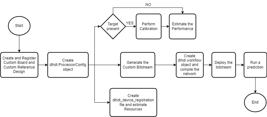
* The clock frequency of the DL processor is: 200MHzThis example shows how to create custom board and generate a deep learning processor IP core for the custom board. In this example you:
Create a custom board and reference design
Estimate the network performance and board resource utilization
Generate a custom processor and bitstream
Deploy the network by using the custom bitstream
The image shows the process of deploying a network to a custom board and retrieving a prediction from the deployed network.
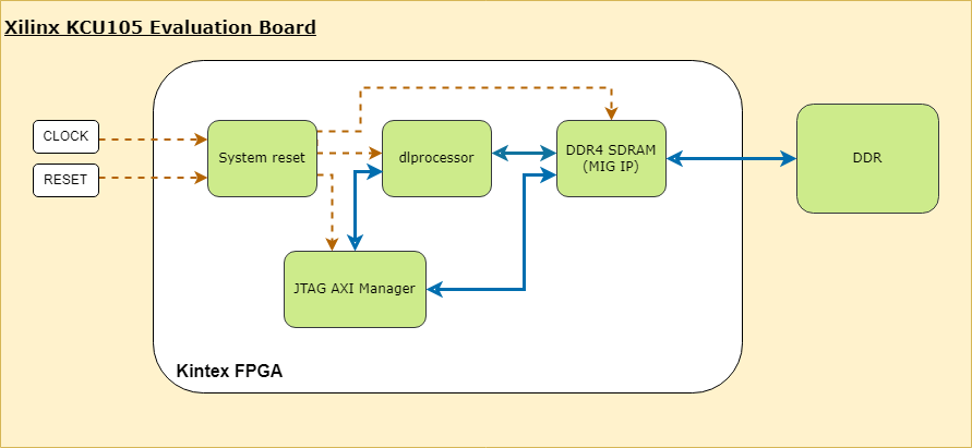
This example uses the Xilinx® Kintex® UltraScale™ KCU105 board. The board contains these blocks:
System reset block — Used to feed the clock and reset signals to the design.
Memory Interface Generator (MIG) IP block — Used to generate memory controllers and interfaces for Xilinx FPGAs.
MATLAB JTAG AXI Manager block — Used by MATLAB to access onboard memory location. For more details, see JTAG AXI Manager (SoC Blockset).
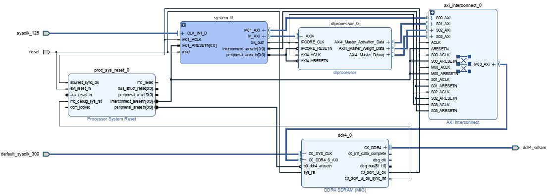
Integrate the generated deep learning processor IP core into your reference design. For more details, see Board and Reference Design Registration System (HDL Coder).
This image shows the generated deep learning processor IP core dl_processor0 integrated into the reference design.
This image shows system_0 block expanded, which contains the "MATLAB as AXI Master" block.
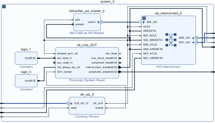
Once the block design is created, export it as a .tcl file.
Register Custom Board
Define the interface and attributes of a custom SoC board. To register the Xilinx® Kintex® UltraScale™ KCU105 board:
1. Create a board registration file with the name hdlcoder_board_customization.m and add it to the MATLAB path. The hdlcoder_board_customization.m function must return a second output. For more information, see Register a Custom Board (HDL Coder).
Set the target workflow to DeepLearningProcessor. For information on other target workflows supported by HDL Coder™, see Workflows in HDL Workflow Advisor (HDL Coder).
function [boardList, workflow] = hdlcoder_board_customization
  % Board plugin registration file
  % 1. Any registration file with this name on MATLAB path will be picked up
  % 2. Registration file returns a cell array pointing to the location of
  %    the board plugins
  % 3. Board plugin must be a package folder accessible from MATLAB path,
  %    and contains a board definition file
  %
  % Copyright 2022-2025 The MathWorks, Inc.
boardList = { ...
     'DLKCU105.plugin_board', ...
      };
workflow = hdlcoder.Workflow.DeepLearningProcessor;
end
2. Create the board definition file. To generate a deep learning processor, you must define the ExternalMemorySize. This property defines the memory size of the DDR on the target board.
% Copyright 2022-2025 The MathWorks, Inc.
% Board definition of KCU105
function hB = plugin_board()
% Construct board object
hB = hdlcoder.Board;
hB.BoardName = 'Xilinx Kintex-Ultrascale KCU105 evaluation board';
% FPGA device information
hB.FPGAVendor   = 'Xilinx';
hB.FPGAFamily   = 'KintexU';
hB.FPGADevice   = 'xcku040-ffva1156-2-e';
hB.FPGAPackage  = '';
hB.FPGASpeed    = '';
% Tool information
hB.SupportedTool = {'Xilinx Vivado'};
% FPGA JTAG chain position
hB.JTAGChainPosition = 1;
% Size of external DDR memory in bytes
hB.ExternalMemorySize = 0x80000000; % 2 GB
% Add interfaces
% Standard "External Port" interface
hB.addExternalPortInterface( ...
    'IOPadConstraint', {'IOSTANDARD = LVCMOS18'});
% Custom board external I/O interface
hB.addExternalIOInterface( ...
     'InterfaceID',    'LEDs General Purpose', ...
     'InterfaceType',  'OUT', ...
     'PortName',       'GPLEDs', ...
     'PortWidth',      8, ...
     'FPGAPin',        {'AP8', 'H23', 'P20', 'P21', 'N22', 'M22', 'R23','P23'}, ...
     'IOPadConstraint', {'IOSTANDARD = LVCMOS18'});
% Custom board external I/O interface
hB.addExternalIOInterface( ...
    'InterfaceID',    'User Push Buttons', ...
    'InterfaceType',  'IN', ...
    'PortName',       'PB', ...
    'PortWidth',      1, ...
    'FPGAPin',        {'AE10'}, ...
    'IOPadConstraint', {'IOSTANDARD = LVCMOS18'});
Register Custom Reference Design
Define the interface and attributes of a custom SoC reference design. To create a custom reference design:
1. Create a reference design registration file named hdlcoder_ref_design_customization.m that contains the list of reference design plugins associated with the board. For more information, see Register a Custom Reference Design (HDL Coder).
function [rd, boardName] = hdlcoder_ref_design_customization
% Reference design plugin registration file
% 1. The registration file with this name inside of a board plugin folder
%    will be picked up
% 2. Any registration file with this name on MATLAB path will also be picked up
% 3. The registration file returns a cell array pointing to the location of
%    the reference design plugins
% 4. The registration file also returns its associated board name
% 5. Reference design plugin must be a package folder accessible from
%    MATLAB path, and contains a reference design definition file
%
%   Copyright 2022-2025 The MathWorks, Inc.
rd = {'DLKCU105.ReferenceDesign.plugin_rd', ...
  };
boardName = 'Xilinx Kintex-Ultrascale KCU105 evaluation board';
end
2. Create the reference design definition file. To generate a deep learning processor IP core, you must define these three AXI4 Master Interfaces:
AXI4 Master Activation DataAXI4 Master Weight DataAXI4 Master Debug
function hRD = plugin_rd()
% Reference design definition
% Copyright 2022-2025 The MathWorks, Inc.
% Construct reference design object
hRD = hdlcoder.ReferenceDesign('SynthesisTool', 'Xilinx Vivado');
hRD.ReferenceDesignName = 'AXI-Stream DDR Memory Access : 3-AXIM';
hRD.BoardName = 'Xilinx Kintex-Ultrascale KCU105 evaluation board';
% Tool information
hRD.SupportedToolVersion = {'2022.1','2023.1','2024.1'};
% Add custom design files
% add custom Vivado design
hRD.addCustomVivadoDesign( ...
  'CustomBlockDesignTcl', 'system_top.tcl',...
  'VivadoBoardPart',      'xilinx.com:kcu105:part0:1.0');
% Add HDL Verifier JTAG as AXI Master IP from support package
hRD.addIPRepository( ...
  'IPListFunction','hdlverifier.fpga.vivado.iplist', ...
  'NotExistMessage', 'IP Repository not found.');
% Add interfaces
% add clock interface
hRD.addClockInterface( ...
     'ClockConnection',      'system_0/clk_out1', ...
     'ResetConnection',      'system_0/peripheral_aresetn',...
     'DefaultFrequencyMHz',  125,...
     'MinFrequencyMHz',      10,...
     'MaxFrequencyMHz',      250,...
     'ClockNumber',          1,...
     'ClockModuleInstance',  'system_0/clk_wiz_0');
% add Register interfaces
% This Register Interface such as AXI4 interface is used for interacting between DDR4 and Deep Learning IP
hRD.addRegisterInterface( ...
    'InterfaceConnection', 'system_0/M_AXI', ...
    'BaseAddress',         '0x44A00000',...
    'MasterAddressSpace',  'system_0/hdlverifier_axi_manager_0/axi4m',...
    'InterfaceType',       'AXI4');
% AXI4 Master Interface for the layer activation data with max data bit-width of 512
hRD.addAXI4MasterInterface(...
        'InterfaceID',         'AXI4 Master Activation Data', ...
        'ReadSupport',          true, ...
        'WriteSupport',         true, ...
        'MaxDataWidth',         512, ...
        'AddrWidth',            32, ...
        'InterfaceConnection', 'axi_interconnect_0/S01_AXI',...
        'TargetAddressSegments', {{'ddr4_0/C0_DDR4_MEMORY_MAP/C0_DDR4_ADDRESS_BLOCK',hex2dec('80000000'),hex2dec('80000000')}});
% AXI4 Master Interface for the layer weight data with max data bit-width of 512
hRD.addAXI4MasterInterface(...
        'InterfaceID',         'AXI4 Master Weight Data', ...
        'ReadSupport',          true, ...
        'WriteSupport',         true, ...
        'MaxDataWidth',         512, ...
        'AddrWidth',            32, ...
        'InterfaceConnection', 'axi_interconnect_0/S02_AXI',...
        'TargetAddressSegments', {{'ddr4_0/C0_DDR4_MEMORY_MAP/C0_DDR4_ADDRESS_BLOCK',hex2dec('80000000'),hex2dec('80000000')}});
% AXI4 Master Interface for the debugger with max data bit-width of 512
hRD.addAXI4MasterInterface(...
        'InterfaceID',         'AXI4 Master Debug', ...
        'ReadSupport',          true, ...
        'WriteSupport',         true, ...
        'MaxDataWidth',         512, ...
        'AddrWidth',            32, ...
        'InterfaceConnection', 'axi_interconnect_0/S03_AXI',...
        'TargetAddressSegments', {{'ddr4_0/C0_DDR4_MEMORY_MAP/C0_DDR4_ADDRESS_BLOCK',hex2dec('80000000'),hex2dec('80000000')}});
3. The reference design plugin file must contain information about the target interface and the deep learning processor IP core, the memory address space for the deep learning processor IP core, and a command to validate the reference design. The file also requires information on the resources consumed by the reference design. This information is used during resource estimation. Add the deep learning processor information to the reference design file:
% Deep learning specific properties
hRD.registerDeepLearningTargetInterface("JTAG");
hRD.registerDeepLearningMemoryAddressSpace(0x80000000, 0x80000000); % 2GB
% Resource utilization information
hRD.ResourcesUsed.LogicElements = 30500;
hRD.ResourcesUsed.DSP = 3;
hRD.ResourcesUsed.RAM = 26.5;
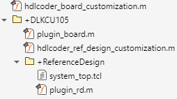
File Hierarchy
The files created need to be saved in the following hierarchy:
Performance Estimation
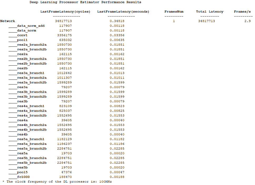
Reduce the time required to design and deploy a custom deep learning network that meets performance requirements by analyzing the layer-level latencies before deploying the network.
Estimate the performance of network for your custom board by collecting calibration data from the custom board, by:
Generating a calibration bitstream
Deploying the calibration bitstream to the target custom board
Retrieving the external to internal memory transaction latencies
Create a Processor Configuration object.
hPC = dlhdl.ProcessorConfig;
Specify the TargetPlatform. This automatically sets the SynthesisToolChipFamily, SynthesisToolDeviceName, and ReferenceDesign properties.
hPC.TargetPlatform = 'Xilinx Kintex-Ultrascale KCU105 evaluation board';
Set the target frequency.
hPC.TargetFrequency = 100;
This example uses a ResNet-18 pretrained network. For more details, see resnet18. Set the deep learning network:
net = imagePretrainedNetwork('resnet18');
To fit this design onto the target, reduce the number of parallel convolution processor kernel threads for the conv module to 9.
setModuleProperty(hPC, 'conv', 'ConvThreadNumber', 9);
Set the Xilinx Vivado toolpath to your design tool using the hdlsetuptoolpath function, then build the calibration bitstream.
hdlsetuptoolpath('ToolName','Xilinx Vivado','ToolPath','C:\Xilinx\Vivado\2024.1\bin\vivado.bat');
bitstreamPath = buildCalibrationBitstream(hPC);
Deploy the bitstream to the hardware and obtain the external- to-internal memory transaction latencies. You can use these values to get better estimates for the layer-level latencies.
deployCalibrationBitstream(hPC, bitstreamPath);
The deployCalibrationBitstream saves the calibration data from the hardware as a structure in the CalibrationData property of the dlhdl.ProcessorConfig object. The function also saves the calibration data as a MAT-file with the name calibrationData.mat. You can load this data into a new dlhdl.ProcessorConfig object by entering:
load('calibrationData.mat');
hPC.CalibrationData = calData;
Estimate the performance of the network for the custom processor configuration.
estimatePerformance(hPC, net);
Resource Estimation
Verify that the generated bistream and network fit on your target custom board, by using estimateResources to estimate the resource utilization. To learn how to estimate the resource utilization for your custom boards, see Estimate Resource Utilization for Custom Board and Reference Design.
Generate Custom Bitstream for Custom Processor Configuration
Generate a bitstream for the custom processor configuration hPC.
dlhdl.buildProcessor(hPC);
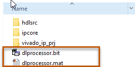
Locate the bitstream file and associated MAT file at cwd\dlhdl_prj\, where cwd is your current working folder. The name of the bitstream file is dlprocessor.bit. The name of the MAT file is dlprocessor.mat. To use the generated bitstream for the supported Xilinx boards, copy the dlprocessor.bit and dlprocessor.mat files to the current working folder.
Deploy the Custom Bitstream and Run Predictions on the Network
After you generate the bitstream, deploy the network and run the predictions on the network. For more information, refer to the Prototype Deep Learning Networks on FPGA and SoC Devices page. For an example on prototyping, see Bicyclist and Pedestrian Classification by Using FPGA.
Create Target Object
Create a target object with the vendor name of the target device. Specify the interface to connect the target device to the host using the Interface name-value pair. This example connects to the target using the JTAG interface.
hT = dlhdl.Target('Xilinx', 'Interface', 'JTAG')
Create Workflow Object for ResNet-18 Network
Create an object of the dlhdl.Workflow class. Specify the network, the bitstream name, and the target object.
hW = dlhdl.Workflow('Network', net, 'Bitstream', 'dlprocessor.bit', 'Target', hT);
Compile the Network
Run the compile function of the dlhdl.Workflow object.
compile(hW)
Deploy the Bitstream to the FPGA
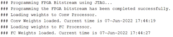
To deploy the network on the Xilinx KCU105 Kintex hardware, run the deploy function of the dlhdl.Workflow object.
deploy(hW)
Run Prediction for the Network
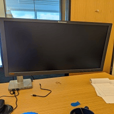
Load the sample image.
img = imread('sampleImage1.png');
imshow(img);
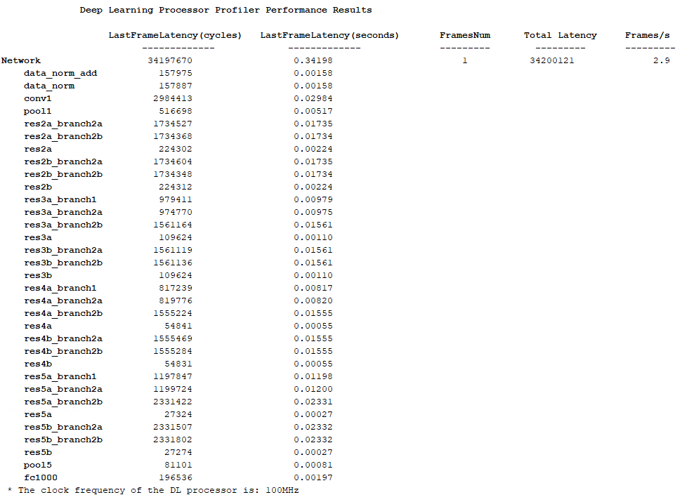
Run a prediction on the image. The result output argument contains the output of the layer preceding the ClassificationOutputLayer and speed contains the profiler table.
[result, speed] = predict(hW, img, 'Profile', 'on');
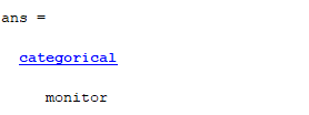
Get the output class from the prediction.
[value,idx] = max(result);
classNames = net.Layers(end).Classes;
classNames(idx)
Limitations
When you estimate the performance Deep Learning HDL Toolbox™ assumes that the deep learning processor is connected to the DDR memory dedicated for the programmable logic (PL) portion of the FPGA or SoC and does not account for the DDR memory communications arbitration with other components.
Tips
To obtain the performance estimation for a dlquantizer object, set the
dlhdl.ProcessorConfig object ProcessorDataType to
int8.
Version History
Introduced in R2021a

